10. Dynamic Programming

This chapter covers the dynamic programming lectures (Weeks 9 and 10). Like divide and conquer (Chapter 2), dynamic programming (DP) solves a problem through smaller versions of it. The difference: in DP the sub-problems overlap, so plain recursion solves the same one again and again. DP solves each sub-problem once, stores the answer, and reuses it. This often turns exponential time into polynomial time.

Fibonacci numbers show the trouble and the fix. A five-step recipe follows, and then it solves two problems: longest common subsequence and 0/1 knapsack.

1. Why Plain Recursion Fails

Divide and conquer: the sub-problems are independent. Mergesort’s two halves share no work. Dynamic programming: the sub-problems overlap. DP adds one rule:

Never compute the answer to the same sub-problem more than once.

Running example: Fibonacci

$$F_0 = 0, \qquad F_1 = 1, \qquad F_n = F_{n-1} + F_{n-2} \quad (n \ge 2).$$

int fib(n) {
    if (n == 0 || n == 1) return n;
    else return fib(n - 1) + fib(n - 2);
}

Each call makes two more calls. The call tree for fib(6) repeats the same values:

That is 25 calls for only 7 different values. (The counts are read off the tree; they are not in the lecture.)

How many calls?

Let $R$ be the number of calls. Bound the tree depth two ways:

• Shortest branch: subtract 2 each time. Every node splits while its argument is at least 2, so the top of the tree is a full binary tree down to depth $n/2$.
• Deepest branch: subtract 1 each time, giving depth $n - 1$.

A full binary tree of depth $D$ has $1 + 2 + \dots + 2^D = 2^{D+1} - 1$ nodes. So

$$2^{n/2 + 1} - 1 < R < 2^n - 1.$$

For $n = 6$: $15 < 25 < 63$. Both bounds are exponential, so plain fib takes $O(2^n)$ time. For $n = 50$ the lower bound alone is about 67 million calls. Only $n + 1$ different sub-problems exist, so almost every call repeats work.

2. The Fix: Store Each Answer

Keep a dictionary (usually an array indexed by sub-problem) of solved answers. Before solving a sub-problem, look it up:

• solved: retrieve the answer in $O(1)$;
• not solved: solve it, then store the answer.

A purple node costs $O(1)$, and the whole sub-tree under it disappears.

DP replaces an exponential-time computation by a polynomial-time one, by storing solutions and never recomputing them.

This is the idea of DFS (Chapter 5): DFS explores only undiscovered vertices, and DP solves only unsolved sub-problems.

Top-down: memoization

Keep the recursion and add the dictionary. Check it before each recursive call. Store the answer just before returning.

int fibDP(n) {
    int f1, f2;
    if (n == 0 || n == 1) { store(Soln, n, n); return n; }
    if (not member(Soln, n - 1)) f1 = fibDP(n - 1);
    else                         f1 = retrieve(Soln, n - 1);
    if (not member(Soln, n - 2)) f2 = fibDP(n - 2);
    else                         f2 = retrieve(Soln, n - 2);
    f1 = f1 + f2;
    store(Soln, n, f1);
    return f1;
}

Soln[0..n] starts at $-1$ (“not solved”). member tests Soln[j] != -1, store sets Soln[j] = s, and retrieve returns Soln[j].

Trace for fibDP(6) (. means still $-1$):

In each call the first value needs a call and the second is retrieved. That prunes the tree.

Cost: one call does constant work, and fibDP really runs once per value $0 \dots n$. Total: $O(n)$, against $O(2^n)$.

3. The Order of Sub-problems

The subproblem graph

• One vertex for each different sub-problem.
• An edge $I \to J$ if solving $I$ makes a recursive call directly on $J$.

The call tree had 25 nodes. The graph has 7 vertices.

• It must be a DAG (Chapter 5). A cycle means a sub-problem needs its own answer.
• Fill order: solve each sub-problem after everything it points to: a reverse topological order. For Fibonacci: $0, 1, \dots, n$.
• Vertices = number of sub-problems = dictionary size.

$$\text{time} \approx (\text{number of sub-problems}) \times (\text{work per sub-problem}).$$

For Fibonacci: $(n+1) \times O(1) = O(n)$. We reuse this formula for every problem below.

Bottom-up: tabulation

Fill the table in that order with loops. No recursion is needed.

soln[0] = 0;
soln[1] = 1;
for j = 2 to n
    soln[j] = soln[j-1] + soln[j-2];

Saving memory. Fibonacci looks back two steps, so two variables are enough: $O(1)$ space. But to rebuild the solution itself (LCS, knapsack), you must keep the whole table.

4. When Is DP Correct? The Principle of Optimality

Many problems ask for the best answer: longest, shortest, most profitable. These are optimization problems. DP is correct for them only if the principle of optimality holds:

The sub-solutions of an optimal solution are themselves optimal solutions of their sub-problems.

Example: if $A \to B \to C \to D$ is a shortest path, then $A \to B \to C$ is a shortest path from $A$ to $C$ (Chapter 6).

DP builds the best answer only from the best answers of smaller problems, never from second-best ones. That is safe only if best solutions are made of best parts.

Cut-and-paste proof. Take an optimal solution. Suppose one part is not optimal for its sub-problem. Paste in a better part. The whole is now better and still valid, which contradicts optimality. Check that the pasted part still fits the rules.

The DP selection rule. When the last decision has several possibilities, compute all of them and take the best. A greedy algorithm (Chapter 6) picks what looks best now and never checks the others.

5. The Five-Step Recipe

Then state the time (formula in Section 3) and the space (table size). Most errors come from step 1: a vague definition leaves step 2 with nothing exact to build on.

6. Longest Common Subsequence (LCS)

A subsequence keeps some characters in their original order, not necessarily adjacent. For ACTTGCG: ACT, AG and ATTC are subsequences. TTA is not (no A after the two Ts). A common subsequence of $x$ and $y$ is a subsequence of both. An LCS is a common subsequence of maximum length. It may not be unique.

Problem. For $x = \langle x_1 \dots x_n \rangle$ and $y = \langle y_1 \dots y_m \rangle$, find the length $LCS(n, m)$. Brute force checks all $2^n$ subsequences of $x$.

Steps 1 and 2: sub-problem and recursion

$LCS(i, j)$ is the length of an LCS of the prefixes $x_1 \dots x_i$ and $y_1 \dots y_j$ ($0 \le i \le n$, $0 \le j \le m$). Prefixes appear because we look at the last character of each, and what remains is a pair of shorter prefixes. Compare $x_i$ with $y_j$:

• $x_i = y_j$. Some LCS ends with this match (standard argument, not in the lecture). Before it must come an LCS of $x_1 \dots x_{i-1}$ and $y_1 \dots y_{j-1}$, or cut-and-paste gives a longer one. Length: $LCS(i-1, j-1) + 1$.
• $x_i \ne y_j$. They cannot both end a common subsequence. So $x_i$ is unused, giving $LCS(i-1, j)$, or $y_j$ is unused, giving $LCS(i, j-1)$. We do not know which, so compute both and take the larger.

$$LCS(i, j) = \begin{cases} 0 & i = 0 \text{ or } j = 0, \\[4pt] LCS(i-1, j-1) + 1 & x_i = y_j, \\[4pt] \max\big(LCS(i-1, j),\; LCS(i, j-1)\big) & x_i \ne y_j. \end{cases}$$

Steps 3 to 5: graph, table, code

Cell $(i, j)$ depends on up-left $(i-1, j-1)$, above $(i-1, j)$ and left $(i, j-1)$.

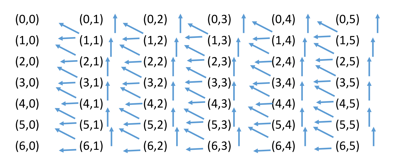
The table c[0..n][0..m] has row 0 and column 0 equal to 0. Fill row by row, left to right, so the three cells are ready.

int LCS(n, m) {
    for i = 0 to n  c[i][0] = 0;
    for j = 1 to m  c[0][j] = 0;
    for i = 1 to n
        for j = 1 to m
            if (x[i] == y[j])
                c[i][j] = c[i-1][j-1] + 1;
            else if (c[i-1][j] >= c[i][j-1])
                c[i][j] = c[i-1][j];
            else
                c[i][j] = c[i][j-1];
    return c[n][m];
}

Cost: $(n+1)(m+1)$ cells at $O(1)$ each. Time $O(nm)$, space $O(nm)$.

Recovering the subsequence

Keep a hint array h that records where each cell’s value came from:

Tie rule: if $c[i-1][j] = c[i][j-1]$, take above (|), because the code tests >=.

Start at h[n][m] and follow the hints back until row 0 or column 0. Each \ gives one character, and they come out last first, so use a stack.

getSequence(n, m) {
    s = empty stack;  i = n;  j = m;
    while (i != 0 and j != 0) {
        if (h[i][j] == '\')       { s.push(x[i]); i--; j--; }
        else if (h[i][j] == '|')  i--;
        else                      j--;
    }
    pop and output everything from s;     // the LCS, in order
}

Each step lowers $i$ or $j$, so the traceback is $O(n + m)$.

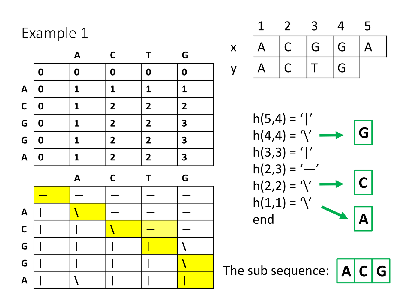
Example 1 (lecture): $x$ = ACGGA, $y$ = ACTG

Five cells in fill order:

• $(1,1)$: A = A, so $c[0][0] + 1 = 1$.
• $(2,2)$: C = C, so $c[1][1] + 1 = 2$.
• $(3,3)$: G $\ne$ T. Above 2, left 2. Tie, take above: 2.
• $(4,4)$: G = G, so $c[3][3] + 1 = 3$.
• $(5,4)$: A $\ne$ G. Above 3, left 2. Take above: 3.

Hint array:

Trace back from $(5,4)$: up to $(4,4)$; \ records G; up from $(3,3)$ to $(2,3)$; left to $(2,2)$; \ records C; \ at $(1,1)$ records A. Reversed, the LCS is ACG, length 3.

Example 2 (lecture): $x$ = CGGTAT, $y$ = AGTTGC

Hint array:

Trace back from $(6,6)$: left, left to $(6,4)$; \ records T; up to $(4,3)$; \ records T; \ at $(3,2)$ records G; then up, up to row 0. Reversed, the LCS is GTT, length 3. Other LCSs of length 3 may exist. The tie rule decides which one is found.

By hand

1. Write $x$ down the side and $y$ across the top. Add a row 0 and a column 0 of zeros.
2. Each cell: if the characters match, take the upper-left value $+1$. Otherwise take the larger of above and left (tie: above).
3. The length is the bottom-right cell. Walk back from there for the subsequence.

7. The 0/1 Knapsack Problem

A knapsack holds total weight at most $C$ (a positive integer). Object $i$ has weight $w_i$ and profit $p_i$ (positive integers). Find the largest total profit of a subset with total weight at most $C$. “0/1” means each object is taken whole or left, never split or repeated. Brute force checks $2^n$ subsets.

Steps 1 and 2: sub-problem and recursion

$P(r, j)$ is the largest profit from the first $j$ objects with capacity $r$ ($0 \le r \le C$, $0 \le j \le n$). The answer is $P(C, n)$. (The lecture writes $C$ for both; $r$ is the variable capacity.) Look at the last object $j$. The best solution takes it or leaves it:

• Take (needs $w_j \le r$): profit $p_j$, capacity left $r - w_j$, so $p_j + P(r - w_j, j-1)$. The rest must be optimal by cut and paste: a better set of weight at most $r - w_j$ still fits with object $j$.
• Leave: $P(r, j-1)$.
• If $w_j > r$, only “leave” is possible.

We do not know which is better, so compute both and take the larger.

$$P(r, 0) = P(0, j) = 0, \qquad P(r, j) = \begin{cases} \max\big(P(r, j-1),\; p_j + P(r - w_j, j-1)\big) & w_j \le r, \\[4pt] P(r, j-1) & w_j > r. \end{cases}$$

Both sub-problems use $j - 1$ objects, so each object is decided once and never taken twice.

Steps 3 to 5: graph, table, code

$(r, j)$ points to $(r, j-1)$ (leave) and $(r - w_j, j-1)$ (take). Every edge lowers $j$, so it is a DAG. Example: $C = 20$ with four objects.

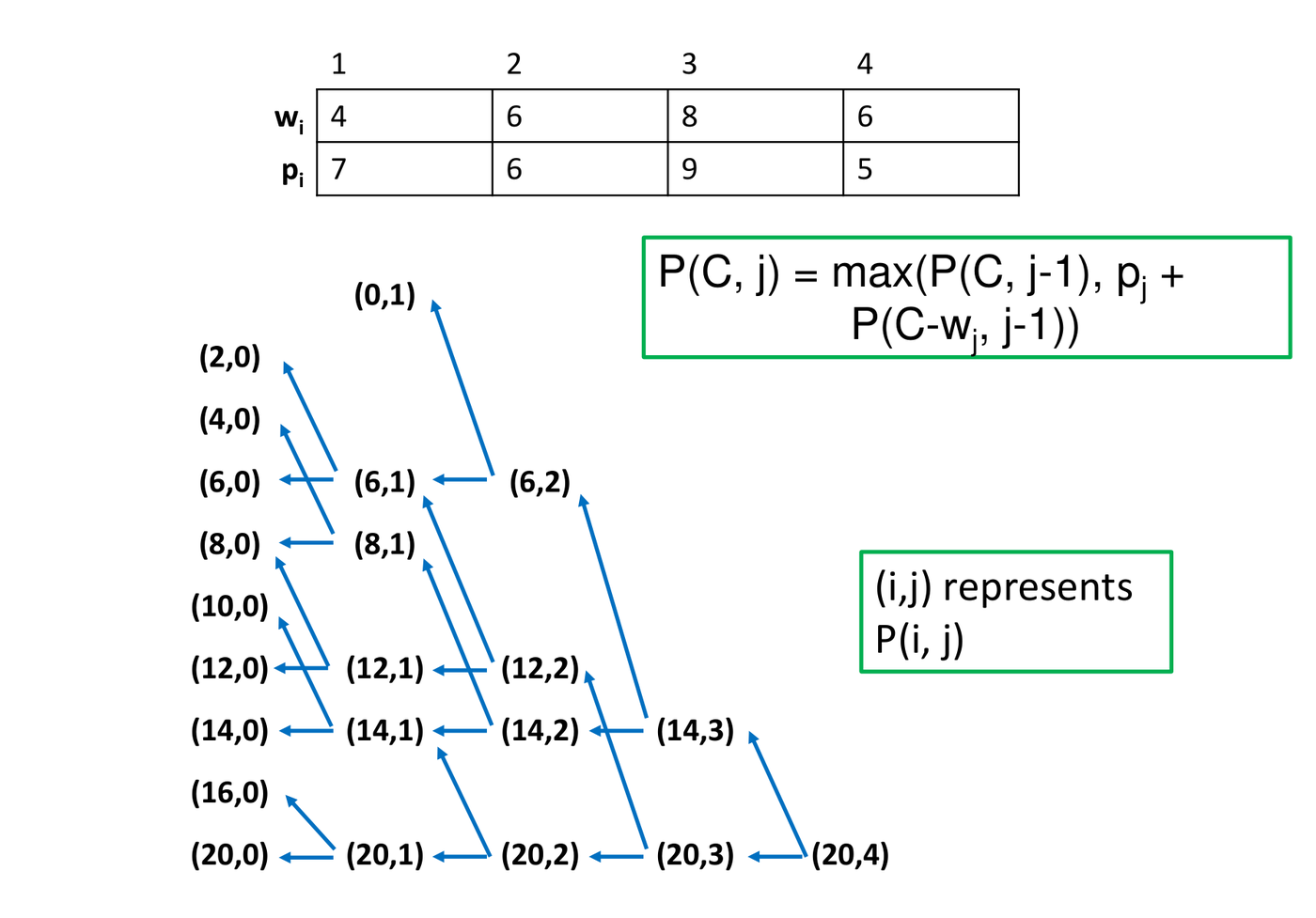
The table profit[C+1][n+1] has rows = capacities and columns = objects. Row 0 and column 0 are 0. Fill so that column $c-1$ is done before column $c$.

int knapsack(int[] w, int[] p, int C, int n) {
    for c = 0 to n  profit[0][c] = 0;
    for r = 1 to C  profit[r][0] = 0;
    for r = 1 to C                         // capacity
        for c = 1 to n {                   // objects 1..c are allowed
            profit[r][c] = profit[r][c-1];                 // leave object c
            if (w[c] <= r)
                if (profit[r][c] < profit[r - w[c]][c-1] + p[c])
                    profit[r][c] = profit[r - w[c]][c-1] + p[c];   // take object c
        }
    return profit[C][n];
}

Example 1 (lecture): $C = 3$

• $(1,2)$: object 2 weighs 2 > 1, so it is left: 1.
• $(2,2)$: leave 1; take $4 + \text{profit}[0][1] = 4$. Best 4.
• $(3,2)$: leave 1; take $4 + \text{profit}[1][1] = 5$. Best 5.
• $(3,3)$: leave 5; take $6 + \text{profit}[0][2] = 6$. Best 6.

The answer is 6: object 3 alone. Objects 1 and 2 together weigh 3 but give only 5.

Example 2 (lecture): $C = 20$

Rows 0 to 3 are all 0 (the lightest object weighs 4).

• $(4,1)$: leave 0; take $7 + 0 = 7$. Best 7.
• $(8,3)$: leave 7; take $9 + \text{profit}[0][2] = 9$. Best 9.
• $(12,2)$: leave 7; take $6 + \text{profit}[6][1] = 13$. Best 13.
• $(18,3)$: leave 13; take $9 + \text{profit}[10][2] = 22$. Best 22.
• $(20,4)$: leave 22; take $5 + \text{profit}[14][3] = 21$. Best 22.

Which objects were taken?

Walk back from $(C, n)$. If $\text{profit}[r][c] = \text{profit}[r][c-1]$, object $c$ was left: go to column $c-1$. Otherwise it was taken: go to row $r - w_c$, column $c-1$. Stop at column 0. (Or store parent pointers while filling.)

Example 2: at $(20,4)$, $22 = $ value at $(20,3)$, so object 4 is left. At $(20,3)$, $22 \ne 13$, so object 3 is taken; go to $(12,2)$. There $13 \ne 7$, so object 2 is taken; go to $(6,1) = 7$, so object 1 is taken. Objects 1, 2, 3: weight $18 \le 20$, profit 22.

Cost: pseudo-polynomial

The table has $(C+1)(n+1)$ cells at $O(1)$ each: time and space $O(nC)$. This is not polynomial in the input size. The size is the number of bits, and $C$ takes only $\log_2 C$ bits to write:

Ten more bits multiply the rows by about 1000. With $b$ bits, $C \approx 2^b$ and the time is about $n \cdot 2^b$: exponential in the input size. An algorithm is pseudo-polynomial if its time is polynomial in the numeric value of the input. Knapsack DP is fast only when $C$ is small.

8. Shortest Paths in a DAG

(Not from the lecture: the slides were not released. This is the standard method.)

1. Sub-problem: $dist(v)$, the shortest distance from the source $s$ to $v$.
2. Recursion: the last edge into $v$ comes from some $u$. By optimality, the path to $u$ is shortest. Try every incoming edge and take the minimum:

$$dist(s) = 0, \qquad dist(v) = \min_{(u, v) \in E} \big(dist(u) + w(u, v)\big).$$

A vertex with no incoming edge (other than $s$) has distance $\infty$.

3. Order: compute in topological order (Chapter 5), so every $u$ is done before $v$.

Cost: each edge is used once, so $O(|V| + |E|)$. Unlike Dijkstra (Chapter 6), this works with negative weights, since a DAG has no cycle. Replace min by max for the longest path.

9. Choosing the Table and the Cost

(General guidance, not from the lecture.)

• A cell that reads a fixed number of cells (Fibonacci 2, LCS 3, knapsack 2) costs $O(1)$.
• A cell that takes a max, min or sum over all smaller values costs $O(n)$. Multiply by the number of cells.
• The plain recursion is usually exponential. To confirm, write its cost as a recurrence and solve it with Chapter 8.

DP, divide and conquer, and greedy

10. Common Traps

• Overlap. DP needs overlapping sub-problems. Without overlap, plain divide and conquer is enough.
• Optimality. DP is correct only if the principle of optimality holds.
• Memoization is top-down, tabulation is bottom-up. Same complexity.
• Order. The subproblem graph must be a DAG. Fill dependencies first (reverse topological).
• Two factors. Time $\approx$ (sub-problems) $\times$ (work per sub-problem). Do not forget the second when a cell loops over many choices.
• Fibonacci. Plain: $O(2^n)$ calls, between $2^{n/2+1}-1$ and $2^n-1$. Memoized: $O(n)$ time. Two variables: $O(1)$ space.
• Define first. Write the sub-problem in words before step 2. A vague step 1 breaks the rest.
• Subsequence vs substring. A subsequence keeps order but need not be contiguous. A substring must be contiguous.
• LCS rules. Match: diagonal $+1$. Mismatch: larger of above and left, never the diagonal. Time and space $O(nm)$, traceback $O(n+m)$. Tie: take above. An LCS may not be unique.
• Memory saving loses the path. Two variables (or two rows) save memory, but you can no longer trace back.
• Knapsack axes. Rows are capacities, columns are objects: profit[r][c].
• Take reads the previous column ($c-1$). Reading the same column lets an object be taken twice.
• Too heavy. If $w_c > r$, “take” does not exist. Do not read a negative row.
• Pseudo-polynomial. $O(nC)$ is not polynomial, because $C$ is a value, not a size.
• Greedy fails. Profit per unit weight does not solve 0/1 knapsack.