1 Vectors

1.1 2-D, 3-D

Scalar: Only magnitude, notation: a,t,x,ya, t, x, y

Vector: Magnitude & direction, notation: f, x, v, w

Vectors v = w if they have the same length & direction.
Origin point does not matter.

image image

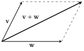
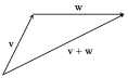
Vector addition: Parallelogram rule and Triangle rule give the same result.

image image

image

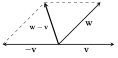
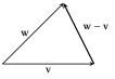
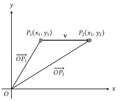
Vector subtraction. ๐’—=P1P2โ†’=P1Oโ†’+OP2โ†’=OP2โ†’โˆ’OP1โ†’\mathbf{v} = \overrightarrow{P_1P_2} = \overrightarrow{P_1O} + \overrightarrow{OP_2} = \overrightarrow{OP_2} - \overrightarrow{OP_1}

image image

Scalar multiple kkv of the vector v is the same whether it is collinear or parallel.

image

๐’—=(v1,v2)\mathbf{v} = (v_1, v_2) or [v1v2]\begin{bmatrix} v_1 \\ v_2 \end{bmatrix}

image

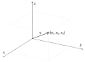
๐’—=(v1,v2,v3)\mathbf{v} = (v_1, v_2, v_3)

Two vectors ๐’—\mathbf{v} = (v1,v2,v3)(v_1, v_2, v_3), ๐’˜\mathbf{w} = (w1,w2,w3)(w_1, w_2, w_3) are equal iff v1=w1,v2=w2,v3=w3v_1 = w_1, v_2 = w_2, v_3 = w_3.

1.2 n-D space

Real line: โ„1\mathbb{R}^1

๐’—โˆˆโ„2:๐’—=(v1,v2)\mathbf{v} \in \mathbb{R}^2: \mathbf{v} = (v_1, v_2)

๐’—โˆˆโ„3:๐’—=(v1,v2,v3)\mathbf{v} \in \mathbb{R}^3: \mathbf{v} = (v_1, v_2, v_3)

๐’—โˆˆโ„n:๐’—=(v1,v2,โ€ฆ,vn)\mathbf{v} \in \mathbb{R}^n: \mathbf{v} = (v_1, v_2, \ldots, v_n) (Set of all ordered n-tuples called n-D space).

Zero vector ๐’—โˆˆโ„n:๐’—=๐ŸŽ=(0,0,โ€ฆ,0)\mathbf{v} \in \mathbb{R}^n: \mathbf{v} = \mathbf{0} = (0, 0, \ldots, 0)

1.2.0.1 Definition

If ๐’—=(v1,v2,โ€ฆ,vn)\mathbf{v} = (v_1, v_2, \ldots, v_n) and ๐’˜=(w1,w2,โ€ฆ,wn)\mathbf{w} = (w_1, w_2, \ldots, w_n) in โ„n\mathbb{R}^n, and for any scalar kk, then

  1. ๐’—+๐’˜=(v1+w1,v2+w2,โ€ฆ,vn+wn)\mathbf{v} + \mathbf{w} = (v_1 + w_1, v_2 + w_2, \ldots, v_n + w_n)

  2. k๐’—=(kv1,kv2,โ€ฆ,kvn)k\mathbf{v} = (kv_1, kv_2, \ldots, kv_n)

  3. โˆ’๐’—=(โˆ’v1,โˆ’v2,โ€ฆ,โˆ’vn)-\mathbf{v} = (-v_1, -v_2, \ldots, -v_n)

  4. ๐’˜โˆ’๐’—=๐’˜+(โˆ’๐’—)=(w1โˆ’v1,w2โˆ’v2,โ€ฆ,wnโˆ’vn)\mathbf{w} - \mathbf{v} = \mathbf{w} + (-\mathbf{v}) = (w_1 - v_1, w_2 - v_2, \ldots, w_n - v_n)

1.2.0.2 Theorem

If ๐’–,๐’—\mathbf{u}, \mathbf{v} and ๐’˜\mathbf{w} are vectors in โ„n\mathbb{R}^n, and if kk and mm are scalars, then

  1. ๐’–+๐’—=๐’—+๐’–\mathbf{u} + \mathbf{v} = \mathbf{v} + \mathbf{u}

  2. (๐’–+๐’—)+๐’˜=๐’–+(๐’—+๐’˜)(\mathbf{u} + \mathbf{v}) + \mathbf{w} = \mathbf{u} + (\mathbf{v} + \mathbf{w})

  3. ๐’–+0=0+๐’–=๐’–\mathbf{u} + 0 = 0 + \mathbf{u} = \mathbf{u}

  4. ๐’–+(โˆ’๐’–)=0\mathbf{u} + (-\mathbf{u}) = 0

  5. k(๐’–+๐’—)=k๐’–+k๐’—k(\mathbf{u} + \mathbf{v}) = k\mathbf{u} + k\mathbf{v}

  6. (k+m)๐’–=k๐’–+m๐’–(k + m)\mathbf{u} = k\mathbf{u} + m\mathbf{u}

  7. k(m๐’–)=(km)๐’–k(m\mathbf{u}) = (km)\mathbf{u}

  8. 1๐’–=๐’–1\mathbf{u} = \mathbf{u}

  9. 0๐’—=00\mathbf{v} = 0

  10. k0=0k0 = 0

  11. โˆ’1๐’—=โˆ’๐’—-1\mathbf{v} = -\mathbf{v}

1.2.0.3 Linear combination

If ๐’˜\mathbf{w} is a vector in โ„n\mathbb{R}^n, then ๐’˜\mathbf{w} is a linear combination of vectors v1,v2,โ€ฆ,vnv_1, v_2,\ldots, v_n in โ„n\mathbb{R}^n if it can be expressed in the from ๐’˜=k1๐’—๐Ÿ+k2๐’—๐Ÿ+โ€ฆ+kn๐’—๐’\mathbf{w} = k_1\mathbf{v_1} + k_2\mathbf{v_2} +\ldots + k_n\mathbf{v_n} where k1,k2,โ€ฆ,knk_1, k_2, \ldots, k_n are scalars and the coefficients of the linear combination.

1.3 Norm, Dot Product and Distance in โ„n\mathbb{R}^n

image

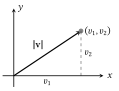
โˆฅ๐’—โˆฅ=v12+v22\|\mathbf{v}\| = \sqrt{v_1^2 + v_2^2}

For a vector ๐’—=(v1,v2,โ€ฆ,vn)\mathbf{v} = (v_1, v_2,\ldots, v_n) in โ„n\mathbb{R}^n, the norm/length/magnitude of ๐’—\mathbf{v} is โˆฅ๐’—โˆฅ=v12+v22+โ€ฆ+vn2\|\mathbf{v}\| = \sqrt{v_1^2 + v_2^2 + \dots + v_n^2}

1.3.0.1 Norm of a vector

For vectors ๐’—\mathbf{v}, ๐’˜\mathbf{w} in โ„n\mathbb{R}^n and a scalar kk,

  1. โˆฅ๐’—โˆฅโ‰ฅ0\|\mathbf{v}\| \geq 0

  2. โˆฅ๐’—โˆฅ=0โ‡”๐’—=0\|\mathbf{v}\| = 0 \iff \mathbf{v} = 0

  3. โˆฅk๐’—โˆฅ=|k|โˆฅ๐’—โˆฅ\|k\mathbf{v}\| = |k|\|\mathbf{v}\|

  4. โˆฅ๐’—+๐’˜โˆฅโ‰คโˆฅ๐’—โˆฅ+โˆฅ๐’˜โˆฅ\|\mathbf{v} + \mathbf{w}\| \leq \|\mathbf{v}\| + \|\mathbf{w}\|

1.3.0.2 Unit vector

For ๐’—\mathbf{v} a nonzero vector in โ„n\mathbb{R}^n, by normalising ๐’—\mathbf{v} we get a unit vector ๐’–\mathbf{u}, with the same direction as ๐’—\mathbf{v}, defined as ๐’–=1โˆฅ๐’—โˆฅ๐’—\mathbf{u} = \frac{1}{\|\mathbf{v}\|}\mathbf{v}

Standard unit vectors are unit vectors that point along the positive axes of the coordinate axes.

In โ„3\mathbb{R}^3, standard unit vectors are ๐’Š=(1,0,0)\mathbf{i} = (1, 0, 0), ๐’‹=(0,1,0)\mathbf{j} = (0, 1, 0), ๐’Œ=(0,0,1)\mathbf{k} = (0, 0, 1).

In โ„n\mathbb{R}^n, we have standard unit vectors

๐’†1=(1,0,0,โ€ฆ,0),๐’†2=(0,1,0,โ€ฆ,0),๐’†3=(0,0,โ€ฆ,1)\mathbf{e}_1 = (1, 0, 0, \ldots, 0), \mathbf{e}_2 = (0, 1, 0, \ldots, 0), \mathbf{e}_3 = (0, 0, \ldots, 1).

1.3.0.3 Distance in โ„n\mathbb{R}^n

For points ๐’–=(u1,u2,โ€ฆ,un)\mathbf{u} = (u_1, u_2, \ldots, u_n), ๐’—=(v1,v2,โ€ฆ,vn)\mathbf{v} = (v_1, v_2, \ldots, v_n) in โ„n\mathbb{R}^n, the distance between ๐’–\mathbf{u} and ๐’—\mathbf{v} is d(๐’–,๐’—)=โˆฅ๐’–โˆ’๐’—โˆฅ=(u1โˆ’v1)2+(u2โˆ’v2)2+โ€ฆ+(unโˆ’vn)2d(\mathbf{u}, \mathbf{v}) = \|\mathbf{u} - \mathbf{v}\| = \sqrt{(u_1 - v_1)^2 + (u_2 - v_2)^2 + \ldots + (u_n - v_n)^2}

Dot Product

For two vectors ๐’–\mathbf{u} and ๐’—\mathbf{v} in โ„n\mathbb{R}^n, their dot product (in geometric form) is ๐’–โ‹…๐’—=โˆฅ๐’–โˆฅโˆฅ๐’—โˆฅcos⁡ฮธ\mathbf{u} \cdot \mathbf{v} = \|\mathbf{u}\|\|\mathbf{v}\|\cos\theta

The component form of the dot product is ๐’–โ‹…๐’—=u1v1+u2v2+โ€ฆ+unvn\mathbf{u} \cdot \mathbf{v} = u_1v_1 + u_2v_2 + \ldots + u_nv_n

Since cos⁡ฮธ=๐’–โ‹…๐’—โˆฅuโˆฅโˆฅvโˆฅ\cos\theta = \frac{\mathbf{u} \cdot \mathbf{v}}{\|u\|\|v\|},

1.3.1 Properties

๐’—โ‹…๐’—=v12+v22+โ€ฆ+vn2=โˆฅvโˆฅ2\mathbf{v} \cdot \mathbf{v} = v_1^2 + v_2^2 + \ldots + v_n^2 = \|v\|^2

We can get length of a vector in terms of its dot product: โˆฅvโˆฅ=๐’—โ‹…๐’—\|v\| = \sqrt{\mathbf{v}\cdot\mathbf{v}}

For vectors ๐’–\mathbf{u}, ๐’—\mathbf{v}, ๐’˜\mathbf{w} in โ„n\mathbb{R}^n and kk a scalar,

  1. ๐’–โ‹…๐’—=๐’—โ‹…๐’–\mathbf{u} \cdot \mathbf{v} = \mathbf{v} \cdot \mathbf{u} [Symmetry]

  2. ๐’–(๐’—+๐’˜)=๐’–โ‹…๐’—+๐’–โ‹…๐’˜\mathbf{u}(\mathbf{v} + \mathbf{w}) = \mathbf{u} \cdot \mathbf{v} + \mathbf{u} \cdot \mathbf{w} [Distributivity]

  3. k(๐’–โ‹…๐’—)=(k๐’–)โ‹…๐’—k(\mathbf{u} \cdot \mathbf{v}) = (k\mathbf{u})\cdot\mathbf{v} [Homogeneity]

  4. ๐’—โ‹…๐’—โ‰ฅ0\mathbf{v}\cdot\mathbf{v} \geq 0 and ๐’—โ‹…๐’—=0โ‡”๐’—=๐ŸŽ\mathbf{v}\cdot\mathbf{v} = 0 \iff \mathbf{v} = \mathbf{0} [Positivity]

  5. ๐ŸŽโ‹…๐’—=๐’—โ‹…๐ŸŽ=0\mathbf{0}\cdot\mathbf{v} = \mathbf{v}\cdot\mathbf{0} = 0

  6. (๐’–+๐’—)โ‹…๐’˜=๐’–โ‹…๐’˜+๐’—โ‹…๐’˜(\mathbf{u} + \mathbf{v})\cdot\mathbf{w} = \mathbf{u}\cdot\mathbf{w} + \mathbf{v}\cdot\mathbf{w}

  7. ๐’–โ‹…(๐’—โˆ’๐’˜)=๐’–โ‹…๐’—โˆ’๐’–โ‹…๐’˜\mathbf{u}\cdot(\mathbf{v} - \mathbf{w}) = \mathbf{u}\cdot\mathbf{v} - \mathbf{u}\cdot\mathbf{w}

  8. (๐’–โˆ’๐’—)โ‹…๐’˜=๐’–โ‹…๐’˜โˆ’๐’—โ‹…๐’˜(\mathbf{u} - \mathbf{v}) \cdot \mathbf{w} = \mathbf{u} \cdot \mathbf{w} - \mathbf{v} \cdot \mathbf{w}

  9. k(๐’–โ‹…๐’—)=๐’–โ‹…(k๐’—)k(\mathbf{u} \cdot \mathbf{v}) = \mathbf{u} \cdot (k\mathbf{v})

1.3.1.1 Cauchy-Schwarz Inequality

If ๐’–=(u1,u2,โ€ฆ,un)\mathbf{u} = (u_1, u_2, \ldots, u_n) and ๐’—=(v1,v2,โ€ฆ,vn)\mathbf{v} = (v_1, v_2, \ldots, v_n) are vectors in โ„n\mathbb{R}^n, then |๐’–โ‹…๐’—|โ‰คโˆฅ๐’–โˆฅโˆฅ๐’—โˆฅ|\mathbf{u}\cdot\mathbf{v}| \leq \|\mathbf{u}\|\|\mathbf{v}\| Hence, โˆ’1โ‰ค๐’–โ‹…๐’—โˆฅ๐’–โˆฅ๐’—โˆฅโ‰ค1-1 \leq \frac{\mathbf{u}\cdot\mathbf{v}}{\|\mathbf{u}\|\mathbf{v}\|} \leq 1, and ฮธ\theta is always defined, where ฮธ=arccos⁡(๐’–โ‹…๐’—โˆฅ๐’–โˆฅ๐’—โˆฅ)\theta = \arccos(\frac{\mathbf{u}\cdot\mathbf{v}}{\|\mathbf{u}\|\mathbf{v}\|}).

1.3.1.2 Triangle Inequality

For vectors ๐’–\mathbf{u}, ๐’—\mathbf{v} and ๐’˜\mathbf{w} in โ„n\mathbb{R}^n and a scalar kk,

  1. โˆฅ๐’–+๐’—โˆฅโ‰คโˆฅ๐’–โˆฅ+โˆฅ๐’—โˆฅ\|\mathbf{u} + \mathbf{v}\| \leq \|\mathbf{u}\| + \|\mathbf{v}\| [For vectors]

  2. d(๐’–,๐’—)โ‰คd(๐’–,๐’˜)+d(๐’˜,๐’—)d(\mathbf{u}, \mathbf{v}) \leq d(\mathbf{u}, \mathbf{w}) + d(\mathbf{w}, \mathbf{v}) [For distances]

1.3.1.3 Orthogonality

Two nonzero vectors ๐’–\mathbf{u} and ๐’—\mathbf{v} in โ„n\mathbb{R}^n are orthogonal if ๐’–โ‹…๐’—=0\mathbf{u}\cdot\mathbf{v} = 0. This means the two vectors are perpendicular to each other, from ฮธ=cos⁡โˆ’1(๐’–โ‹…๐’—โˆฅuโˆฅโˆฅvโˆฅ)\theta = \cos^{-1}\left(\frac{\mathbf{u}\cdot\mathbf{v}}{\|u\|\|v\|}\right) A nonempty set of vectors in โ„n\mathbb{R}^n is an orthogonal set if all pairs of distinct vectors in the set are orthogonal.

Equations of lines and planes

image

image

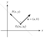
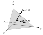
For point-normal equations, we need two things:

  1. Coordinates of a point on the line/plane, P0P_0.

  2. The normal from that point, ๐’\mathbf{n}, which is orthogonal to the line/plane.

We make use of the property ๐’โ‹…P0Pโ†’=0\mathbf{n}\cdot\overrightarrow{P_0P} = 0, where PP is the variable point of the line/plane.

For a line (in โ„n\mathbb{R}^n): ๐’โ‹…P0Pโ†’=0P0Pโ†’=(xโˆ’x0,yโˆ’y0)๐’=(a,b)a(xโˆ’x0)+b(yโˆ’y0)=0\begin{align*} \mathbf{n} \cdot \overrightarrow{P_0P} &= 0 \\ \overrightarrow{P_0P} &= (x - x_0, y - y_0) \\ \mathbf{n} &= (a, b) \\ a(x - x_0) + b(y - y_0) &= 0 \end{align*}

For a plane: ๐’โ‹…P0Pโ†’=0P0Pโ†’=(xโˆ’x0,yโˆ’y0,zโˆ’z0)๐’=(a,b,c)a(xโˆ’x0)+b(yโˆ’y0)+c(zโˆ’z0)=0\begin{align*} \mathbf{n} \cdot \overrightarrow{P_0P} &= 0 \\ \overrightarrow{P_0P} &= (x - x_0, y - y_0, z - z_0) \\ \mathbf{n} &= (a, b, c) \\ a(x - x_0) + b(y - y_0) + c(z - z_0) &= 0 \end{align*}

If ax+by+cz=0ax + by + cz = 0, then the line/plane passes through the origin.
Note that the coefficients of the line/plane are the normal vector values.

Vector/Parametric Equations

image

image

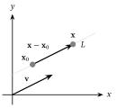
For a line containing point x0x_0 and parallel to vector ๐’—\mathbf{v}, the vector form is ๐’™โˆ’๐’™๐ŸŽ=t๐’—\mathbf{x} - \mathbf{x_0} = t\mathbf{v} and the parametric form is x=x0+tay=y0+tbz=z0+tc\begin{align*} x &= x_0 + ta \\ y &= y_0 + tb \\ z &= z_0 + tc \end{align*}

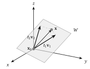
For a vector containing point x0x_0 and parallel to noncollinear vectors v1v_1 and v2v_2, the vector form is ๐’™โˆ’๐’™0=t1๐’—1+t2๐’—2\mathbf{x} - \mathbf{x}_0 = t_1\mathbf{v}_1 + t_2\mathbf{v}_2 and the parametric form is x=x0+t1a1+t2a2x=y0+t1b1+t2b2x=z0+t1c1+t2c2\begin{align*} x &= x_0 + t_1a_1 + t_2a_2 \\ x &= y_0 + t_1b_1 + t_2b_2 \\ x &= z_0 + t_1c_1 + t_2c_2 \end{align*}

If ๐’™0\mathbf{x}_0 is ๐ŸŽ\mathbf{0}, then the line/plane passes through the origin.

2 Matrices

2.1 Notation

A square matrix, AA, of order nn has nn columns and nn rows.

Then, trace A=a11+a22+โ€ฆ+ann\text{trace } A = a_{11} + a_{22} + \ldots + a_{nn}

A diagonal matrix is a square matrix where all entries off the main diagonal are 0.

If AA is a diagonal matrix, A=[a1100โ‹ฏ00a220โ‹ฏ000a33โ‹ฏ0โ‹ฎโ‹ฎโ‹ฎโ‹ฑ00000ann]A = \begin{bmatrix} a_{11} & 0 & 0 & \cdots & 0 \\ 0 & a_{22} & 0 & \cdots & 0 \\ 0 & 0 & a_{33} & \cdots & 0 \\ \vdots & \vdots & \vdots & \ddots & 0\\ 0 & 0 & 0 & 0 & a_{nn} \end{bmatrix}

If AA is an identity/unit matrix, A=[100โ‹ฏ0010โ‹ฏ0001โ‹ฏ0โ‹ฎโ‹ฎโ‹ฎโ‹ฑ000001]A = \begin{bmatrix} 1 & 0 & 0 & \cdots & 0 \\ 0 & 1 & 0 & \cdots & 0 \\ 0 & 0 & 1 & \cdots & 0 \\ \vdots & \vdots & \vdots & \ddots & 0\\ 0 & 0 & 0 & 0 & 1 \end{bmatrix}

The transpose of an mร—nm\times n matrix AA is an nร—mn\times m matrix ATA^T.

(AT)T=A(A^T)^T = A. A=[a11a12โ‹ฏa1na21a22โ‹ฏa2nโ‹ฎโ‹ฎโ‹ฑโ‹ฎam1am2โ‹ฏamn],AT=[a11a21โ‹ฏam1a12a22โ‹ฏam2โ‹ฎโ‹ฎโ‹ฑโ‹ฎa1na2nโ‹ฏamn]A = \begin{bmatrix} a_{11} & a_{12} & \cdots & a_{1n} \\ a_{21} & a_{22} & \cdots & a_{2n} \\ \vdots & \vdots & \ddots & \vdots \\ a_{m1} & a_{m2} & \cdots & a_{mn} \end{bmatrix}, \quad A^T = \begin{bmatrix} a_{11} & a_{21} & \cdots & a_{m1} \\ a_{12} & a_{22} & \cdots & a_{m2} \\ \vdots & \vdots & \ddots & \vdots \\ a_{1n} & a_{2n} & \cdots & a_{mn} \end{bmatrix}

If AA is a symmetric matrix, then AT=AA^T = A, and aij=ajia_{ij} = a_{ji}. A=[173745352]A = \begin{bmatrix} 1 & 7 & 3 \\ 7 & 4 & 5 \\ 3 & 5 & 2 \end{bmatrix}

If AA is a skew-symmetric matrix, then AT=โˆ’AA^T = -A, and aij=โˆ’ajia_{ij} = -a_{ji}.

Diagonal elements must be zero, because each element must be its own negative. A=[02โˆ’45โˆ’20โˆ’44540],AโŠค=[0โˆ’245204โˆ’45โˆ’40]=โˆ’A.A = \begin{bmatrix} 0 & 2 & -45 \\ -2 & 0 & -4 \\ 45 & 4 & 0 \end{bmatrix}, \quad A^\top = \begin{bmatrix} 0 & -2 & 45 \\ 2 & 0 & 4 \\ -45 & -4 & 0 \end{bmatrix} = -A.

2.1.1 Example

Let YY be an arbitrary 3ร—33\times3 non-zero skew-symmetric matrix and ZZ be an arbitrary 3ร—33\times3 non-zero symmetric matrix. Is Y3Z4โˆ’Z4โˆ’Y3Y^3Z^4-Z^4-Y^3 symmetric?

Note: AkA^k, where kk is a scalar, refers to Aร—Aโ‹ฏAA\times A \cdots A for kk times.

If k=0k=0, then A0=IA^0 = I, the identity matrix.

We have that

First, we find the transpose of Y3Y^3 and Z4Z^4: (Y3)T=(YT)3=(โˆ’Y)3=โˆ’Y3(Z4)T=(ZT)4=Z4\begin{align*} (Y^3)^T &= (Y^T)^3 = (-Y)^3 = -Y^3 \\ (Z^4)^T &= (Z^T)^4 = Z^4 \end{align*}

Let A=Y3Z4โˆ’Z4Y3A = Y^3Z^4 - Z^4Y^3. We calculate ATA^T: AT=(Y3Z4โˆ’Z4Y3)T=(Y3Z4)Tโˆ’(Z4Y3)T=(Z4)T(Y3)Tโˆ’(Y3)T(Z4)T=(Z4)(โˆ’Y3)โˆ’(โˆ’Y3)(Z4)=โˆ’Z4Y3+Y3Z4=Y3Z4โˆ’Z4Y3=A\begin{align*} A^T &= (Y^3Z^4 - Z^4Y^3)^T \\ &= (Y^3Z^4)^T - (Z^4Y^3)^T \tag{Distributive property} \\ &= (Z^4)^T (Y^3)^T - (Y^3)^T (Z^4)^T \tag{Reversal law} \\ &= (Z^4)(-Y^3) - (-Y^3)(Z^4) \tag{Substitution} \\ &= -Z^4Y^3 + Y^3Z^4 \\ &= Y^3Z^4 - Z^4Y^3 \\ &= A \end{align*}

Since AT=AA^T = A, the matrix is symmetric.

2.2 Operations

Define mร—nm\times n matrices A=[aij],B=[bij],C=[cij]A = [a_{ij}], B=[b_{ij}], C=[c_{ij}].

For two matrices AA and BB to be equal,

  1. AA and BB are of same size, mร—nm\times n

  2. aij=bija_{ij} = b_{ij} for 1โ‰คiโ‰คm1\leq i\leq m and 1โ‰คjโ‰คn1\leq j\leq n

Addition and subtraction of matrices require matrices of similar sizes and are calculated entrywise.

i.e. For C=A+BC=A+B, cij=aij+bijc_{ij} = a_{ij} + b_{ij}.

Scalar multiplication multiplies each entry by a scalar ss.

i.e. For C=sAC=sA, cij=sโ‹…aijc_{ij} = s\cdot a_{ij}.

Basic properties:

Matrix Multiplication

If AA is an mร—nm\times n matrix and BB is an nร—pn\times p matrix, then the product C=ABC = AB is an mร—pm\times p matrix. cij=ai1b1j+ai1b1j+โ€ฆ+ainbnj=โˆ‘k=1naikbkjc_{ij} = a_{i1}b_{1j} + a_{i1}b_{1j} +\ldots + a_{in}b_{nj} = \sum_{k=1}^{n}a_{ik}b_{kj}

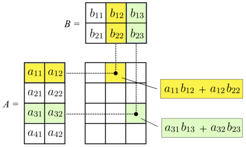
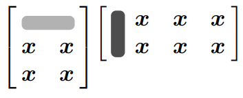
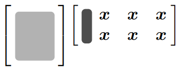
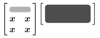
Visualisation of matrix multiplication
(Row ii of A)โ‹…\cdot(Column kk of B) = Each number cikc_{ik} in ABAB
Dot Product method

Properties:

More properties involving vectors:

Matrix Multiplication by columns AB=A[๐’ƒ1๐’ƒ2โ‹ฏ๐’ƒp]=[A๐’ƒ1A๐’ƒ2โ‹ฏA๐’ƒp]AB = A\begin{bmatrix} \bm{b}_1 & \bm{b}_2 & \cdots & \bm{b}_p \end{bmatrix} = \begin{bmatrix} A\bm{b}_1 & A\bm{b}_2 & \cdots & A\bm{b}_p \end{bmatrix}

Aโ‹…A \cdot(Column kk of B) = Column kk of ABAB

Matrix Multiplication by rows AB=[๐’‚1๐’‚2โ‹ฎ๐’‚m]B=[๐’‚1B๐’‚2Bโ‹ฎ๐’‚mB]AB = \begin{bmatrix} \bm{a}_1 \\ \bm{a}_2 \\ \vdots \\ \bm{a}_m \end{bmatrix} B = \begin{bmatrix} \bm{a}_1 B \\ \bm{a}_2 B \\ \vdots \\ \bm{a}_m B \end{bmatrix}

(Row ii of A)โ‹…B\cdot B = Row ii of ABAB

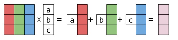
Matrix multiplication as linear combination

Linear combination of column vectors of AA, where the coefficients are elements of the single column vector.

Example:

Let A=[1234]A = \begin{bmatrix} 1 & 2 \\ 3 & 4 \end{bmatrix} and B=[5678]B = \begin{bmatrix} 5 & 6 \\ 7 & 8 \end{bmatrix}

Method 1: Multiply AA with each column in BB, producing a column of ABAB.

A๐’ƒ1=[1234][57]=[row 1โ‹…๐’ƒ1row 2โ‹…๐’ƒ1]=[1โ‹…5+2โ‹…73โ‹…5+4โ‹…7]=[1943]A\bm{b}_1 = \begin{bmatrix} 1 & 2 \\ 3 & 4 \end{bmatrix} \begin{bmatrix} 5 \\ 7 \end{bmatrix} = \begin{bmatrix} \text{row } 1 \cdot \bm{b}_1 \\ \text{row } 2 \cdot \bm{b}_1 \end{bmatrix} = \begin{bmatrix} 1 \cdot 5 + 2 \cdot 7 \\ 3 \cdot 5 + 4 \cdot 7 \end{bmatrix} = \begin{bmatrix} 19 \\ 43 \end{bmatrix}

A๐’ƒ2=[1234][68]=[row 1โ‹…๐’ƒ2row 2โ‹…๐’ƒ2]=[1โ‹…6+2โ‹…83โ‹…6+4โ‹…8]=[2250]A\bm{b}_2 = \begin{bmatrix} 1 & 2 \\ 3 & 4 \end{bmatrix} \begin{bmatrix} 6 \\ 8 \end{bmatrix} = \begin{bmatrix} \text{row } 1 \cdot \bm{b}_2 \\ \text{row } 2 \cdot \bm{b}_2 \end{bmatrix} = \begin{bmatrix} 1 \cdot 6 + 2 \cdot 8 \\ 3 \cdot 6 + 4 \cdot 8 \end{bmatrix} = \begin{bmatrix} 22 \\ 50 \end{bmatrix}

AB=[19224350]AB = \begin{bmatrix} 19 & 22 \\ 43 & 50 \end{bmatrix}

Method 2: Multiple each row in AA with BB, producing a row of ABAB. ๐’‚1B=[12][5678]=[1โ‹…5+2โ‹…71โ‹…6+2โ‹…8]=[1922]\bm{a}_1B = \begin{bmatrix} 1 & 2 \end{bmatrix} \begin{bmatrix} 5 & 6 \\ 7 & 8 \end{bmatrix} = \begin{bmatrix} 1\cdot5 + 2\cdot7 & 1\cdot6 + 2\cdot8 \end{bmatrix} = \begin{bmatrix} 19 & 22 \end{bmatrix} ๐’‚2B=[34][5678]=[3โ‹…5+4โ‹…73โ‹…6+4โ‹…8]=[4350]\bm{a}_2B = \begin{bmatrix} 3 & 4 \end{bmatrix} \begin{bmatrix} 5 & 6 \\ 7 & 8 \end{bmatrix} = \begin{bmatrix} 3\cdot5 + 4\cdot7 & 3\cdot6 + 4\cdot8 \end{bmatrix} = \begin{bmatrix} 43 & 50 \end{bmatrix} AB=[19224350]AB = \begin{bmatrix} 19 & 22 \\ 43 & 50 \end{bmatrix}

Method 3: Each column ii of ABAB as a linear combination of columns of AA, with coefficients from corresponding column ii of BB. ๐’„1=5[13]+7[24]=[1943]\begin{aligned} \bm{c}_1 &= 5 \begin{bmatrix} 1 \\ 3 \end{bmatrix} + 7 \begin{bmatrix} 2 \\ 4 \end{bmatrix} = \begin{bmatrix} 19 \\ 43 \end{bmatrix} \end{aligned} ๐’„2=6[13]+8[24]=[2250]\begin{aligned} \bm{c}_2 &= 6 \begin{bmatrix} 1 \\ 3 \end{bmatrix} + 8 \begin{bmatrix} 2 \\ 4 \end{bmatrix} = \begin{bmatrix} 22 \\ 50 \end{bmatrix} \end{aligned}

Example

If the order of AA is 4ร—34\times3, BB is 4ร—54\times5 and CC is 7ร—37\times3, then what is the order of (ATB)TCT(A^TB)^TC^T?

(ATB)TCT=(BT(AT)T)CT=BTACT=(5ร—4โ‹…4ร—3)ร—(3ร—7)=(5ร—3)ร—(3ร—7)=๐Ÿ“ร—๐Ÿ•\begin{align*} (A^T B)^T C^T &= (B^T (A^T)^T) C^T \\ &= B^T A C^T \\ &= (5 \times 4 \cdot 4 \times 3) \times (3 \times 7) \\ &= (5 \times 3) \times (3 \times 7) \\ &= \mathbf{5 \times 7} \end{align*}

Inverse of a matrix

An nร—nn\times n square matrix AA is invertible if โˆƒ\exists an nร—nn\times n square matrix BB s.t. AB=BA=InAB = BA = I_n where InI_n is the nร—nn\times n identity matrix.

For a 2ร—22\times2 square matrix [abcd]\begin{bmatrix} a & b \\ c & d \end{bmatrix}, it is invertible if and only if det⁡(A)=|A|=adโˆ’bcโ‰ 0\det(A) = |A| = ad - bc \neq 0 and the inverse of A is denoted by Aโˆ’1=1adโˆ’bc[dโˆ’bโˆ’ca]A^{-1} = \frac{1}{ad-bc}\begin{bmatrix} d & -b \\ -c & a \end{bmatrix}

If det⁡(A)=0\det(A) = 0, then AA is singular and is non-invertible.

If AA and BB are invertible matrices of the same size, then ABAB is invertible, and (AB)โˆ’1=Bโˆ’1Aโˆ’1(AB)^{-1} = B^{-1}A^{-1}

If AA is invertible, then ATA^T is invertible, and (AT)โˆ’1=(Aโˆ’1)T(A^T)^{-1} = (A^{-1})^T