10 Complex Numbers

10.1 Basics

A complex number $z$ is defined as $$z = a + ib$$ where $j$ or $i = \sqrt{-1}$.
Re($z$) = a, Im($z$) = b.
By Fundamental Theorem of Algebra, every polynomial of degree $n$ is now guaranteed to have exactly $n$ roots. For example, a quadratic equation will always yield two roots—if they aren’t real, they will be complex.

10.1.1 Algebra w/ $i$

$i^1 = i$, $i^2 = -1$, $i^3 = -i$, $i^4 = 1$.
Inverse of $i$: $\frac{1}{i} = -i$.

The rule $\sqrt{A}\sqrt{B} = \sqrt{AB}$ only works if at least one of the numbers is positive.
If both are negative, we have to pull the $i$ out first.
For example, find $\sqrt{-4}\sqrt{-9}$. Wrong way is: $\sqrt{-4}\sqrt{-9} = \sqrt{-4\cdot -9} =\sqrt{36} = 6$.
Instead, do $\sqrt{-4}\sqrt{-9} = i\sqrt{4}\cdot i\sqrt{9} = 2i\cdot 3i = 6i^2 = -6$.

10.1.2 Representing complex numbers

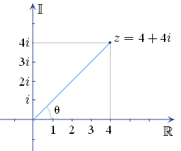
3 ways to represent complex numbers:

1. Rectangular/Cartesian form: $z = a + ib$.
   Best for addition/subtraction, and geometrically represents vector addition.

   • Multiplication: $z_1 \cdot z_2 = (a_1a_2 - b_1b_2) + i(b_1a_2 + a_1b_2)$

   • Division: $\frac{z_1}{z_2} = \frac{a_1a_2 + b_1b_2}{a_2^2 + b_2^2} + j\frac{b_1a_2 - a_1b_2}{a_2^2 + b_2^2}$

2. Polar form $z = r\angle\theta = \cos\theta + i\sin\theta$.
   The modulus is $r = |z| = \sqrt{a^2 + b^2}$.
   The argument is $\theta$, measured anti-clockwise from the positive real axis.

   • Because angles loop every $2\pi$ radians ($360^\circ$), an argument isn’t uniquely defined. To fix this, Principal Argument is limited to the range $(-\pi, \pi]$.

3. Exponential $z = re^{i\theta}$.
   Best for multiplication/division.

   • Multiplication: $z_1z_2 = (r_1 \cdot r_2)e^{i(\theta_1 + \theta_2)}$

   • Division: $\frac{z_1}{z_2} = \frac{r_1}{r_2}e^{i(\theta_1 - \theta_2)}$

10.1.3 Complex conjugate

The complex conjugate of $z = a + ib$ is $$\overline{z} = a - ib$$ Geometrically, this complex vector is reflected in the Real axis.

• $z\cdot\bar{z} = a^2 + b^2$.

• $\overline{z_1 + z_2} = \overline{z}_1 + \overline{z}_2$, and $\overline{(z_1z_2)} = \overline{z}_1\overline{z}_2$

10.2 De Moivre’s Theorem

Euler’s formula: $$e^{i\theta} = \cos(\theta) + i\sin(\theta)$$ De Moivre’s Theorem: For a complex number $z$ and any integer $n$, $$z^n = (r e^{i\theta})^n = r^n e^{in\theta} = r^n(\cos(n\theta) + i\sin(n\theta))$$ De Moivre’s Theorem applied to roots:
$$z^{1/n} = r^{1/n} e^{j(\frac{\theta + 2\pi k}{n})} \quad \text{for } k = 0, 1, \dots, n-1$$ So taking the $n$-th root of a complex number will give $n$ distinct angles.

Example Find $(1+j)^{-1/3}$.
First convert to exponential form. Magnitude $r = \sqrt{1^2 + 1^2} = \sqrt{2} = 2^{1/2}$. Angle $\theta = \arctan(\frac{1}{1}) = \pi/4$.
Hence $1+j = \sqrt{2}e^{j\pi/4}$.
Then we have $$z_k = (\sqrt{2})^{-1/3} e^{j(\frac{\pi/4 + 2\pi k}{-3})} \quad \text{for } k = 0, 1, 2$$ Then for $k=0$, $z_0 = 2^{-1/6} e^{-j\pi/12}$, for $k=1$, $z_1 = 2^{-1/6} e^{-j3\pi/4}$, and for $k=2$, $z_2 = 2^{-1/6} e^{j7\pi/12}$.
Geoemetrically, the three roots are spaced $\frac{2\pi}{3}$ radians apart on a circle of radius 0.89.

10.3 Discrete Fourier Transform (DFT)

10.3.1 Complex exponentials & vectors

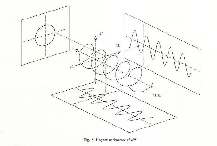
Think of complex numbers as moving geometric objects.
A complex exponential like $e^{i\theta}$ can be thought of as a rotating clock hand in the argand plane, around the centre.
$$e^{i\theta} = e^{i\omega n}$$ Replacing the static angle $\theta$ with $\omega n$, where $\omega$ can be thought of as the angular frequency (how many radians per sample) and $n$ is the sample we are measuring.
A complex vector then represents snapshots of the rotating clock hand. For example, a vector like $z = \begin{bmatrix} 1 & i & -1 & -i \end{bmatrix}^\top$ tell us that at each time-step ($n$ increasing by 1), we rotate anti-clockwise by $\frac{\pi}{2}$ radians.
Further, stack these 2D snapshots on top of each other, and pull them forward along a time axis. We get a 3D spiral.

10.3.2 Inner product and inverse of complex matrices

If we have a complex vector like $\begin{bmatrix} 1 & i \end{bmatrix}^\top$, and taking the dot product with itself, we get $1 + (-1) = 0$, which is impossible as the length of that vector is non-zero.
Instead, if we multiply a complex number with its conjugate, like $(a+ib)(a-ib) = a^2 + b^2$, we get the positive result desired.
Therefore, the inner product of complex vectors $\mathbf{a}$ and $\mathbf{b}$ is $$\langle a, b \rangle = b^H a$$ where $\mathbf{b}^H$ (Hermitian/conjugate transpose) transposes $\mathbf{b}$ and takes the conjugate of every imaginary number in it.
In the context of DFT, the inner product reveals the relationship between some signal wave and a basis wave. Two complex vectors are considered to be pointing in the same direction if they are rotating at the exact same frequency.
If the inner product outputs 0, the signal vector has zero component in the direction of the basis vector (orthogonal). In DFT, this means the specific frequency does not exist in the signal.
Otherwise, the complex scalar output reveals the magnitude and phase-shift to shift the signal wave so as to align it to the basis vector.

10.3.3 The real meat

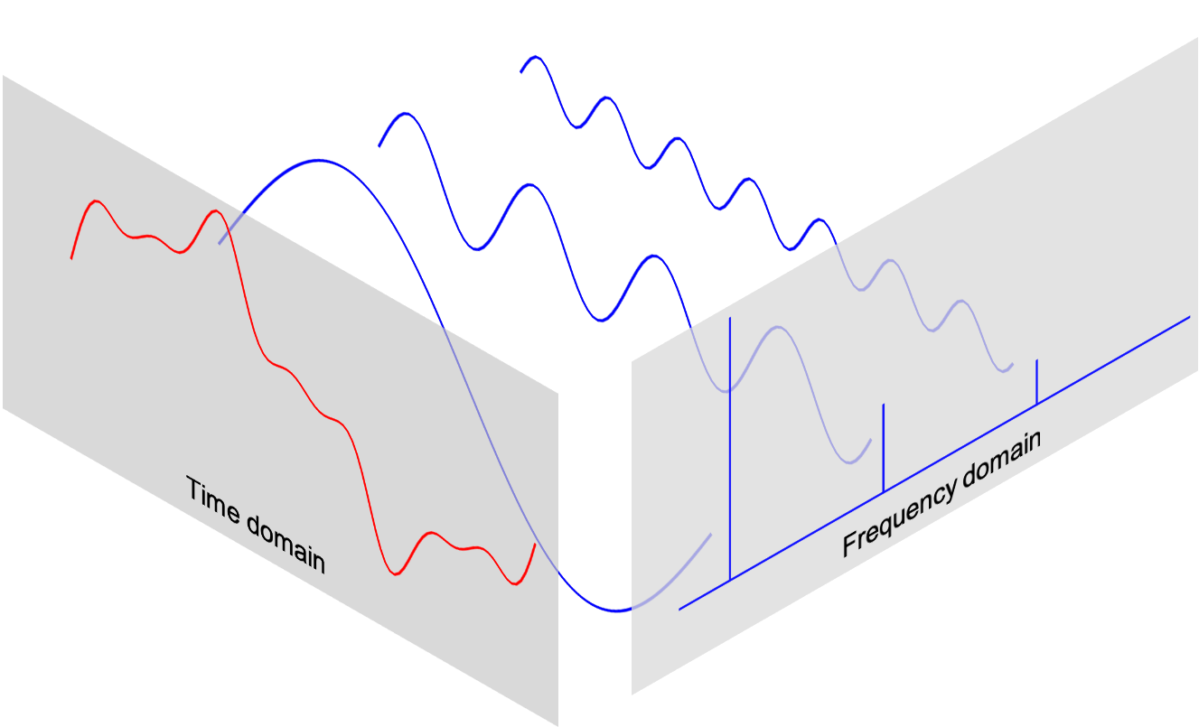
The idea of DFT is that any discrete time-signal $x[n]$ of length $N$ can be decomposed into/rebuilt using $N$ basic waves.

The original signal is $x[n]$ of length $N$. This means we sampled $N$ discrete times from the original signal, and the values form the vector of $N$ complex numbers.

How to represent the basic waves?
Each basis vector contains $N$ complex numbers (same as the original signal).
We generate a basis vector for every harmonic frequency. There are $N$ of these basis vectors (indexed by $k = 0, 1, \ldots, N-1$).
So to build the $k$-th basis vector, we take $N$ time-steps through that basis vector, using the formula: $$e_k[n] = e^{i\frac{2\pi}{N}kn}$$ Each basis vector thus looks like this: $$e_k = \begin{bmatrix} e^{i\frac{2\pi}{N}k(0)} \\ e^{i\frac{2\pi}{N}k(1)} \\ e^{i\frac{2\pi}{N}k(2)} \\ \vdots \\ e^{i\frac{2\pi}{N}k(N-1)} \end{bmatrix}$$
We use that specific complex exponential because:

• By Euler’s formula ($\cos + i\sin$), it packages a cosine and sine wave, so we can encapsulate the amplitude and phase.

• Notice that the "angular frequency" $\omega = \frac{2\pi}{N}k$. So when step $n=N$, we get $\exp^{2\pi k}$, when is 1 (the starting point). It is thus periodic around $N$.

• $k$ is the frequency index. It determines how many $2\pi$ full cycles we complete over $N$ steps. E.g. $k=2$ basis wave spins twice as fast as $k=1$ basis wave. The magic is that two waves with different $k$ will have their peaks and valleys perfectly misaligned in a balanced way. When you take the inner product of both waves, we get exactly 0.

• The magnitude is 1 for every term, so multiplying the signal by these basis vectors only act as a rotational tool.

As noted above, every basis vector is orthogonal to each other. $$\begin{align*} \langle e_k, e_m \rangle &= \sum_{n=0}^{N-1} e^{i\frac{2\pi}{N}kn} \cdot e^{-i\frac{2\pi}{N}mn}\\ &= \sum_{n=0}^{N-1} e^{i\frac{2\pi}{N}(k-m)n}\\ &= 0 \quad [\text{taking $N$ evenly spaced points around a circle,}\\ & \quad \text{and adding them up, will cancel each other out}] \end{align*}$$
Forward DFT (Analysis)
Forward DFT is breaking down the messy signal to find the frequencies that make up that signal.
From $x$, we want $X$, a column vector of $N$ frequency bins. Each term in $X$, denoted as $X[k]$ is a complex number.
The magnitude $|X[k]|$ tells us the amplitude of that specific frequency, and the phase $\angle X[k]$ tells us how much it is shifted left or right.
$$X = \begin{bmatrix} X[0] \\ X[1] \\ X[2] \\ \vdots \\ X[N-1] \end{bmatrix} = \begin{bmatrix} \text{DC Offset (0 Hz)} \\ \text{1st Harmonic} \\ \text{2nd Harmonic} \\ \vdots \\ \text{Highest frequency} \end{bmatrix}$$ The forward DFT has the following matrix equation: $$X = Wx$$ $W$ is an $N \times N$ matrix. Representing $W_N = e^{-j\frac{2\pi}{N}}$, the formula for any term in $W$ is just $W_N^{kn}$, at row $k$ and column $n$. $$\begin{align*} W &= \begin{bmatrix} W_N^{0\cdot0} & W_N^{0\cdot1} & W_N^{0\cdot2} & \dots & W_N^{0\cdot(N-1)} \\ W_N^{1\cdot0} & W_N^{1\cdot1} & W_N^{1\cdot2} & \dots & W_N^{1\cdot(N-1)} \\ W_N^{2\cdot0} & W_N^{2\cdot1} & W_N^{2\cdot2} & \dots & W_N^{2\cdot(N-1)} \\ \vdots & \vdots & \vdots & \ddots & \vdots \\ W_N^{(N-1)\cdot0} & W_N^{(N-1)\cdot1} & W_N^{(N-1)\cdot2} & \dots & W_N^{(N-1)\cdot(N-1)} \end{bmatrix}\\ &= \begin{matrix} \begin{matrix} n \text{ increases } \longrightarrow \end{matrix} \\ \begin{bmatrix} 1 & 1 & 1 & \dots & 1 \\ 1 & e^{-i\frac{2\pi}{N}(1)(1)} & e^{-i\frac{2\pi}{N}(1)(2)} & \dots & e^{-i\frac{2\pi}{N}(1)(N-1)} \\ 1 & e^{-i\frac{2\pi}{N}(2)(1)} & e^{-i\frac{2\pi}{N}(2)(2)} & \dots & e^{-i\frac{2\pi}{N}(2)(N-1)} \\ \vdots & \vdots & \vdots & \ddots & \vdots \\ 1 & e^{-i\frac{2\pi}{N}(N-1)(1)} & e^{-i\frac{2\pi}{N}(N-1)(2)} & \dots & e^{-i\frac{2\pi}{N}(N-1)(N-1)} \end{bmatrix} \begin{matrix} k \\ \text{increases} \\ \downarrow \end{matrix} \end{matrix} \end{align*}$$
Note that every row is one basis vector/wave.
The exponents are negative so as to take the complex conjugate of the actual basis vector, for valid inner products. However, intuitively, if a signal contains some harmonic $k$, it is spinning anti-clockwise at speed of $\frac{2\pi}{N}k$. Our basis vector should then spin in the opposite direction (negative exponent) at the same speed, effectively unwinding that specific frequency. Mathematically, $$e^{i\theta}\cdot e^{-i\theta} = e^0 = 1$$ Then adding up all the constant values, we get a massive spike for that frequency bin.
On the other hand, if the test wave spins at different speeds, it doesn’t perfectly unwind the signal, and the positive and negative peaks cancel out to 0.

By basic matrix multiplication, the $k$-th entry of $X$, $X[k]$ is the inner product of the $k$-th row of $W$ and the column vector $x$. Hence we get the summation form of the forward DFT: $$X[k] = \sum_{n=0}^{N-1} x[n] e^{-i \frac{2\pi}{N} kn}$$ Hence, we get $X$ from $x$ using $W$, the matrix of basis vectors. Note that $W$ is fixed, and we can construct $W$ (from the complex exponential) so long as we know $N$ (from length of $x$).

Backward DFT (Synthesis)
Now we have $X$, the mix of different frequencies, and we want to get back $x$, the original signal.
The matrix equation here is: $$x = \frac{1}{N} W^H X$$ Recall that $W^H$ is the conjugate transpose of $W$.
The exponents are positive, i.e. $\exp^{i\frac{2\pi}{N}kn}$. Also, the columns of $W^H$ are now the basis vectors.
So $x$ is the linear combination of the columns of $W^H$, and $X$ provides the weights to scale each corresponding frequency by.
Note that we need to multiply by $\frac{1}{N}$. Since $W^H\cdot W = NI$, and $X = Wx$, hence $\frac{1}{N}W^H\cdot W x = x$ balances the equation.
Each term of $W^H$ is now $$e^{i\frac{2\pi}{N}k n}$$ and the full matrix $W^H$ is $$W^H = \begin{matrix} \begin{matrix} k \text{ increases } \longrightarrow \end{matrix} \\ \begin{bmatrix} 1 & 1 & 1 & \dots & 1 \\ 1 & e^{i\frac{2\pi}{N}(1)(1)} & e^{i\frac{2\pi}{N}(2)(1)} & \dots & e^{i\frac{2\pi}{N}(N-1)(1)} \\ 1 & e^{i\frac{2\pi}{N}(1)(2)} & e^{i\frac{2\pi}{N}(2)(2)} & \dots & e^{i\frac{2\pi}{N}(N-1)(2)} \\ \vdots & \vdots & \vdots & \ddots & \vdots \\ 1 & e^{i\frac{2\pi}{N}(1)(N-1)} & e^{i\frac{2\pi}{N}(2)(N-1)} & \dots & e^{i\frac{2\pi}{N}(N-1)(N-1)} \end{bmatrix} \begin{matrix} n \\ \text{increases} \\ \downarrow \end{matrix} \end{matrix}$$ By matrix multiplication, the $n$-th entry of $x$ is obtained by taking inner product of $n$-th row of $W^H$ and the column vector $X$. I.e. the sum of all same time snapshot $n$ across all the different frequencies.

A note on the matrix $W$, as we progress down the rows, $k$ increases. The waves spin faster.
For a purely real-valued $x$, $$X[N-k] = \overline{X[k]}$$ I.e. frequencies that are symmetrical around the $N/2$ point look like negative frequencies (spinning backwards).
Hence, a real-valued signal $x$ has unique information in rows 0 to $N/2$, while rows $N/2 + 1$ to $N-1$ are redundant.
If $x$ is complex, every single one of the $N$ rows is unique and necessary