8 Orthogonality

Recall that two nonzero vectors $\mathbf{u}$, $\mathbf{v}$ $\in$ $\mathbb{R}^n$ are orthogonal if $$\mathbf{u}\cdot\mathbf{v}=0$$ The zero vector is orthogonal to every vector in $\mathbb{R}^n$.
$\mathbf{u}\cdot\mathbf{v}=0 \iff \theta = \frac{\pi}{2}$, where $\theta = \frac{\mathbf{u}\cdot\mathbf{v}}{\|\mathbf{u}\|\|\mathbf{v}\|}$.

8.1 Orthogonal Complements

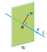
If a vector $\mathbf{z}$ is orthogonal to every vector in a subspace $W$ in $\mathbb{R}^n$, then $\mathbf{z}$ is orthogonal to $W$.
The set of all vectors $z$ that are orthogonal to $W$ is the orthogonal complement of $W$, denoted by $W^\perp$.

1. Vector $\mathbf{x} \in W \iff \mathbf{x}$ is orthogonal to every vector in a set that spans $W$.

   • Only need to check if $\mathbf{x}$ is perpendicular to the vectors that span $W$ (its basis vectors).

2. $W^\perp$ is a subspace of $\mathbb{R}^n$.

   • $W^\perp$ contains the zero vector and is closed under addition and scalar multiplication.

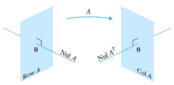
An $m \times n$ matrix $A$ acts as a linear transformation mapping vectors from a domain ($\mathbb{R}^n$) to a codomain ($\mathbb{R}^m$).
We have the following relationships: $$(\text{Row } A)^\perp = \text{Nul } A \quad \text{and} \quad (\text{Col } A)^\perp = \text{Nul } A^T$$ Proof.

1. $\text{Nul } A \subseteq (\text{Row } A)^\perp$: If a vector $\mathbf{x}$ is in $\text{Nul } A$, then $A\mathbf{x} = \mathbf{0}$. When you compute $A\mathbf{x}$, you are taking the dot product of each row of $A$ with the vector $\mathbf{x}$. Because the result is a zero vector, $\mathbf{x}$ must be orthogonal to every single row of $A$. Because the rows of $A$ span $\text{Row } A$, $\mathbf{x}$ is orthogonal to the entire row space.

2. $(\text{Row } A)^\perp \subseteq \text{Nul } A$: If we start with a vector $\mathbf{x}$ that is orthogonal to $\text{Row } A$, it must inherently be orthogonal to each individual row of $A$. Therefore, the dot product of each row with $\mathbf{x}$ is $0$, meaning $A\mathbf{x} = \mathbf{0}$. This confirms $\mathbf{x}$ is in $\text{Nul } A$.

3. Substituting $A^T$ into the first rule gives: $(\text{Row } A^T)^\perp = \text{Nul } A^T \implies (\text{Col } A)^\perp = \text{Nul } A^T$.

8.2 Orthogonal Projections

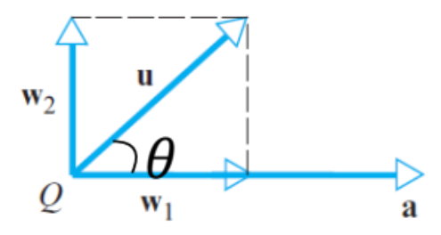
Sometimes, we need to break a vector $\mathbf{u}$ into two orthogonal vectors relative to reference vector $\mathbf{a}$.

8.2.0.1 Projection Theorem

We can express $\mathbf{u}$ exactly one way as $$\mathbf{u} = \mathbf{w}_1 + \mathbf{w}_2$$ where $\mathbf{w}_1$ is a scalar multiple of $\mathbf{a}$, and $\mathbf{w}_2$ is a vector orthogonal to $\mathbf{a}$.
$\mathbf{w}_1$ is the orthogonal projection of $\mathbf{u}$ onto $\mathbf{a}$. $$\text{proj}_\mathbf{a} \mathbf{u} = \left( \frac{\mathbf{u} \cdot \mathbf{a}}{\|\mathbf{a}\|^2} \right) \mathbf{a} = \left( \frac{\mathbf{u}\cdot\mathbf{a}}{\|\mathbf{a}\|}\right) \frac{\mathbf{a}}{\|\mathbf{a}\|} = \|\mathbf{u}\|\cos\theta \cdot \hat{\mathbf{a}}$$ $\mathbf{w}_2$ is vector component of $\mathbf{u}$ orthogonal to $\mathbf{a}$ (or the residual). $$\mathbf{w}_2 = \mathbf{u} - \text{proj}_\mathbf{a} \mathbf{u}$$ The norm of the projection is $$\|\text{proj}_\mathbf{a} \mathbf{u}\| = \frac{|\mathbf{u} \cdot \mathbf{a}|}{\|\mathbf{a}\|} = \|\mathbf{u}\| |\cos \theta|$$

8.2.0.2 Pythagoras’ Theorem in $\mathbb{R}^n$

If $\mathbf{u}$ and $\mathbf{v}$ are orthogonal vectors, then $$\|\mathbf{u} + \mathbf{v}\|^2 = \|\mathbf{u}\|^2 + \|\mathbf{v}\|^2$$ Proof. $$\|\mathbf{u} + \mathbf{v}\|^2 = (\mathbf{u} + \mathbf{v}) \cdot (\mathbf{u} + \mathbf{v}) = \|\mathbf{u}\|^2 + 2(\mathbf{u} \cdot \mathbf{v}) + \|\mathbf{v}\|^2 = \|\mathbf{u} + \mathbf{v}\|^2 = \|\mathbf{u}\|^2 + \|\mathbf{v}\|^2$$

8.3 Orthogonal Sets & Bases

A set of vectors $\{\mathbf{u}_1, \dots, \mathbf{u}_p\}$ in $\mathbb{R}^n$ is said to be an orthogonal set if each pair of distinct vectors from the set is orthogonal. Mathematically, this means their dot product is zero: $$\mathbf{u}_i \cdot \mathbf{u}_j = 0 \quad \text{whenever} \quad i \neq j$$

8.3.0.1 Theorem

If $S = \{\mathbf{u}_1, \dots, \mathbf{u}_p\}$ is an orthogonal set of nonzero vectors in $\mathbb{R}^n$, then $S$ is linearly independent and hence is an orthogonal basis for the subspace spanned by $S$.
Note that $p \leq n$. If $p=n$, then $S$ is an orthogonal basis for the entire space $\mathbb{R}^n$.
Note also that not all bases are orthogonal.
Proof. Assume there is a linear combination that equals the zero vector: $$\mathbf{0} = c_1\mathbf{u}_1 + \dots + c_p\mathbf{u}_p$$ If we take the dot product of both sides with $\mathbf{u}_1$: $$\mathbf{0} \cdot \mathbf{u}_1 = (c_1\mathbf{u}_1 + c_2\mathbf{u}_2 + \dots + c_p\mathbf{u}_p) \cdot \mathbf{u}_1$$ $$0 = c_1(\mathbf{u}_1 \cdot \mathbf{u}_1) + c_2(\mathbf{u}_2 \cdot \mathbf{u}_1) + \dots + c_p(\mathbf{u}_p \cdot \mathbf{u}_1)$$ Because $S$ is an orthogonal set, all dot products where $i \neq j$ are zero. This leaves: $$0 = c_1(\mathbf{u}_1 \cdot \mathbf{u}_1)$$ Since $\mathbf{u}_1$ is a nonzero vector, $\mathbf{u}_1 \cdot \mathbf{u}_1$ is not zero. Therefore, $c_1$ must be $0$. By repeating this for each vector, all weights $c_i$ must be zero, proving the set is linearly independent.

8.3.1 Computing Coordinates Relative to an Orthogonal Basis

8.3.1.1 Theorem

Let $\{\mathbf{u}_1, \dots, \mathbf{u}_p\}$ be an orthogonal basis for a subspace $W$ of $\mathbb{R}^n$. For each $\mathbf{y}$ in $W$, the weights in the linear combination $\mathbf{y} = c_1\mathbf{u}_1 + \dots + c_p\mathbf{u}_p$ are given by: $$c_j = \frac{\mathbf{y} \cdot \mathbf{u}_j}{\mathbf{u}_j \cdot \mathbf{u}_j} \quad (j = 1, \dots, p)$$ The proof for this is similar to the above theorem.

8.3.2 Orthogonal Projections onto Subspaces

8.3.2.1 Theorem

Let $W$ be a subspace of $\mathbb{R}^n$. Then each $\mathbf{y}$ in $\mathbb{R}^n$ can be written uniquely in the form: $$\mathbf{y} = \hat{\mathbf{y}} + \mathbf{z}$$ where $\hat{\mathbf{y}}$ is in $W$ and $\mathbf{z}$ is in $W^\perp$ (orthogonal to $W$).
If $\{\mathbf{u}_1, \dots, \mathbf{u}_p\}$ is any orthogonal basis of $W$, then the orthogonal projection of $\mathbf{y}$ onto $W$ (denoted as $\hat{\mathbf{y}}$ or $\text{proj}_W \mathbf{y}$) is calculated as: $$\hat{\mathbf{y}} = \left(\frac{\mathbf{y} \cdot \mathbf{u}_1}{\mathbf{u}_1 \cdot \mathbf{u}_1}\right)\mathbf{u}_1 + \dots + \left(\frac{\mathbf{y} \cdot \mathbf{u}_p}{\mathbf{u}_p \cdot \mathbf{u}_p}\right)\mathbf{u}_p$$ and the residual is $\mathbf{z} = \mathbf{y} - \hat{\mathbf{y}}$.
Example: Let $\{\mathbf{u}_1, \dots, \mathbf{u}_5\}$ be an orthogonal basis for $\mathbb{R}^5$ and let $\mathbf{y} = c_1\mathbf{u}_1 + \dots + c_5\mathbf{u}_5$. Consider the subspace $W = \text{Span}\{\mathbf{u}_1, \mathbf{u}_2\}$. Write $\mathbf{y}$ as the sum of a vector $\mathbf{z}_1$ in $W$ and a vector $\mathbf{z}_2$ in $W^\perp$.
Naturally, group the terms based on the orthogonal basis: $$\mathbf{y} = \underbrace{c_1\mathbf{u}_1 + c_2\mathbf{u}_2}_{\mathbf{z}_1} + \underbrace{c_3\mathbf{u}_3 + c_4\mathbf{u}_4 + c_5\mathbf{u}_5}_{\mathbf{z}_2}$$

1. $\mathbf{z}_1$ is clearly in $\text{Span}\{\mathbf{u}_1, \mathbf{u}_2\}$ (which is $W$).

2. To prove $\mathbf{z}_2$ is in $W^\perp$, we must show it is orthogonal to the basis of $W$. Let’s check against $\mathbf{u}_1$: $$\mathbf{z}_2 \cdot \mathbf{u}_1 = (c_3\mathbf{u}_3 + c_4\mathbf{u}_4 + c_5\mathbf{u}_5) \cdot \mathbf{u}_1 = c_3(\mathbf{u}_3 \cdot \mathbf{u}_1) + c_4(\mathbf{u}_4 \cdot \mathbf{u}_1) + c_5(\mathbf{u}_5 \cdot \mathbf{u}_1) = 0$$ A similar calculation shows $\mathbf{z}_2 \cdot \mathbf{u}_2 = 0$. Thus, $\mathbf{z}_2$ is in $W^\perp$.

8.4 Orthonormal Sets & Orthogonal Matrices

8.4.1 Orthonormal sets

A set of vectors $\{\mathbf{u}_1, \dots, \mathbf{u}_p\}$ is an orthonormal set if it is an orthogonal set of unit vectors. $$\mathbf{u}_i \cdot \mathbf{u}_j = 0 \quad (\text{for } i \neq j) \quad \text{and} \quad \mathbf{u}_i \cdot \mathbf{u}_i = 1$$ If an orthonormal set spans a subspace $W$, it is an orthonormal basis for $W$. (It is automatically linearly independent.)
The simplest example: The standard basis in $\mathbb{R}^n$ (e.g., $\mathbf{e}_1, \mathbf{e}_2, \dots, \mathbf{e}_n$) is an orthonormal basis.
Example: Show that $\{\mathbf{v}_1, \mathbf{v}_2, \mathbf{v}_3\}$ is an orthonormal basis of $\mathbb{R}^3$, where: $\mathbf{v}_1 = \begin{bmatrix} 3/\sqrt{11} \\ 1/\sqrt{11} \\ 1/\sqrt{11} \end{bmatrix}$, $\mathbf{v}_2 = \begin{bmatrix} -1/\sqrt{6} \\ 2/\sqrt{6} \\ 1/\sqrt{6} \end{bmatrix}$, $\mathbf{v}_3 = \begin{bmatrix} -1/\sqrt{66} \\ -4/\sqrt{66} \\ 7/\sqrt{66} \end{bmatrix}$.

1. Check orthogonality: $\mathbf{v}_1 \cdot \mathbf{v}_2 = -3/\sqrt{66} + 2/\sqrt{66} + 1/\sqrt{66} = 0$, and so on.

2. Check unit length: $\mathbf{v}_1 \cdot \mathbf{v}_1 = 9/11 + 1/11 + 1/11 = 1$ and so on.

Hence it is an orthonormal set.

8.4.2 Matrices with Orthonormal Columns

8.4.2.1 Theorem

An $m \times n$ matrix $U$ has orthonormal columns if and only if $U^T U = I$.
Proof. When you multiply $U^T U$, the entry in row $i$ and column $j$ is the dot product of column $\mathbf{u}_i$ and column $\mathbf{u}_j$.

• If $i = j$ (the diagonal entries), $\mathbf{u}_i^T \mathbf{u}_i = 1$ (because they are unit vectors).

• If $i \neq j$ (the off-diagonal entries), $\mathbf{u}_i^T \mathbf{u}_j = 0$ (because they are orthogonal).

$$U^T U = \begin{bmatrix} \leftarrow \mathbf{u}_1^T \rightarrow \\ \leftarrow \mathbf{u}_2^T \rightarrow \\ \vdots \\ \leftarrow \mathbf{u}_n^T \rightarrow \end{bmatrix} \begin{bmatrix} \uparrow & \uparrow & & \uparrow \\ \mathbf{u}_1 & \mathbf{u}_2 & \dots & \mathbf{u}_n \\ \downarrow & \downarrow & & \downarrow \end{bmatrix} = \begin{bmatrix} \mathbf{u}_1 \cdot \mathbf{u}_1 & \mathbf{u}_1 \cdot \mathbf{u}_2 & \dots & \mathbf{u}_1 \cdot \mathbf{u}_n \\ \mathbf{u}_2 \cdot \mathbf{u}_1 & \mathbf{u}_2 \cdot \mathbf{u}_2 & \dots & \mathbf{u}_2 \cdot \mathbf{u}_n \\ \vdots & \vdots & \ddots & \vdots \\ \mathbf{u}_n \cdot \mathbf{u}_1 & \mathbf{u}_n \cdot \mathbf{u}_2 & \dots & \mathbf{u}_n \cdot \mathbf{u}_n \end{bmatrix}$$ If the original vectors were orthonormal, it simplifies to: $$U^T U = \begin{bmatrix} 1 & 0 & \dots & 0 \\ 0 & 1 & \dots & 0 \\ \vdots & \vdots & \ddots & \vdots \\ 0 & 0 & \dots & 1 \end{bmatrix} = I$$

8.4.2.2 Theorem

Let $U$ be an $m \times n$ matrix with orthonormal columns, and let $\mathbf{x}$ and $\mathbf{y}$ be vectors in $\mathbb{R}^n$. Transforming vectors via $U$ preserves their lengths and their relationships to one another:

1. Preserves Length: $\|U\mathbf{x}\| = \|\mathbf{x}\|$

2. Preserves Dot Product: $(U\mathbf{x}) \cdot (U\mathbf{y}) = \mathbf{x} \cdot \mathbf{y}$

3. Preserves Orthogonality: $(U\mathbf{x}) \cdot (U\mathbf{y}) = 0$ if and only if $\mathbf{x} \cdot \mathbf{y} = 0$

Proof. Property 2: $(U\mathbf{x}) \cdot (U\mathbf{y}) = (U\mathbf{x})^T (U\mathbf{y}) = \mathbf{x}^T U^T U \mathbf{y} = \mathbf{x}^T I \mathbf{y} = \mathbf{x}^T \mathbf{y} = \mathbf{x} \cdot \mathbf{y}$.
Property 1 follows as such: $\|U\mathbf{x}\|^2 = (U\mathbf{x}) \cdot (U\mathbf{x}) = \mathbf{x} \cdot \mathbf{x} = \|\mathbf{x}\|^2$.
Example: Let $U = \begin{bmatrix} 1/\sqrt{2} & 2/3 \\ 1/\sqrt{2} & -2/3 \\ 0 & 1/3 \end{bmatrix}$ and $\mathbf{x} = \begin{bmatrix} \sqrt{2} \\ 3 \end{bmatrix}$. Verify that $\|U\mathbf{x}\| = \|\mathbf{x}\|$.
$$U\mathbf{x} = \begin{bmatrix} 1/\sqrt{2} & 2/3 \\ 1/\sqrt{2} & -2/3 \\ 0 & 1/3 \end{bmatrix} \begin{bmatrix} \sqrt{2} \\ 3 \end{bmatrix} = \begin{bmatrix} 1 + 2 \\ 1 - 2 \\ 0 + 1 \end{bmatrix} = \begin{bmatrix} 3 \\ -1 \\ 1 \end{bmatrix}$$ Compare norms:

• $\|U\mathbf{x}\| = \sqrt{3^2 + (-1)^2 + 1^2} = \sqrt{9 + 1 + 1} = \sqrt{11}$

• $\|\mathbf{x}\| = \sqrt{(\sqrt{2})^2 + 3^2} = \sqrt{2 + 9} = \sqrt{11}$

8.4.3 Orthogonal matrices

If a matrix has orthonormal columns AND is square, it is an orthogonal matrix.
A orthogonal matrix $Q$ is a real square matrix, whose columns and rows are orthonormal vectors.

• $Q^T Q = Q Q^T = I$.

• $Q^T = Q^{-1}$.

Reason: $Q$ is square, so its left inverse is also its right inverse, forcing $QQ^T = I$. Just as $Q^TQ$ computes the dot products of the columns, $QQ^T$ computes the dot products of the rows: $$QQ^T = \begin{bmatrix} \leftarrow \mathbf{r}_1 \rightarrow \\ \leftarrow \mathbf{r}_2 \rightarrow \\ \vdots \end{bmatrix} \begin{bmatrix} \uparrow & \uparrow & \\ \mathbf{r}_1^T & \mathbf{r}_2^T & \dots \\ \downarrow & \downarrow & \end{bmatrix} = \begin{bmatrix} \mathbf{r}_1 \cdot \mathbf{r}_1 & \mathbf{r}_1 \cdot \mathbf{r}_2 \\ \mathbf{r}_2 \cdot \mathbf{r}_1 & \mathbf{r}_2 \cdot \mathbf{r}_2 \end{bmatrix} = \begin{bmatrix} 1 & 0 \\ 0 & 1 \end{bmatrix}$$ Geometrically, if $Q$ is $n \times n$ orthogonal matrix, there are $n$ orthogonal columns in a $n$-D space, hence forming a basis for the entire space.
A classic $2 \times 2$ orthogonal matrix $Q$ is $$Q = \begin{bmatrix} \cos(30^\circ) & -\sin(30^\circ) \\ \sin(30^\circ) & \cos(30^\circ) \end{bmatrix} = \begin{bmatrix} \sqrt{3}/2 & -1/2 \\ 1/2 & \sqrt{3}/2 \end{bmatrix}$$

• Column 1: Imagine taking the standard $x$-axis and rotating counter-clockwise $30^\circ$. Length is still 1.

• Column 2: Same thing for the $y$-axis.

If matrix $U$ is $m \times n$ matrix, and $m > n$, it is NOT an orthogonal matrix.
$U^T U = I$ is still true, yielding an $n \times n$ identity matrix.
But $U U^T$ yields an $m \times m$ matrix $\neq I$. Instead, $P = U U^T$ creates an $m \times m$ projection matrix of rank $n$. This matrix $P$ can be used to project any given vector $\mathbf{y}$ onto the column space of $U$ (let’s call it $W$) using the formula: $\hat{\mathbf{y}} = U U^T \mathbf{y} = P\mathbf{y}$. Geometrically, for example if $m=3$, $n=2$, the two vectors span a flat 2D plane cutting through that 3D space.

8.5 Orthogonal Decomposition

Generalising an earlier theorem in 1-D space to higher-dimensional space,

8.5.0.1 Theorem

Let $W$ be a subspace of $\mathbb{R}^n$. Then each $\mathbf{y}$ in $\mathbb{R}^n$ can be written uniquely in the form: $$\mathbf{y} = \hat{\mathbf{y}} + \mathbf{z}$$

• $\hat{\mathbf{y}}$ is entirely inside the subspace $W$, it is the orthogonal projection of $\mathbf{y}$ onto $W$, written as $\text{proj}_W \mathbf{y}$.

• $\mathbf{z}$ is in $W^\perp$ (orthogonal to every vector in $W$), it is calculated as $\mathbf{z} = \mathbf{y} - \hat{\mathbf{y}}$.

Formula: If $\{\mathbf{u}_1, \dots, \mathbf{u}_p\}$ is any orthogonal basis of $W$, then: $$\hat{\mathbf{y}} = \left(\frac{\mathbf{y} \cdot \mathbf{u}_1}{\mathbf{u}_1 \cdot \mathbf{u}_1}\right)\mathbf{u}_1 + \dots + \left(\frac{\mathbf{y} \cdot \mathbf{u}_p}{\mathbf{u}_p \cdot \mathbf{u}_p}\right)\mathbf{u}_p$$ Proof. We have the residual $\mathbf{z} = \mathbf{y} - \hat{\mathbf{y}}$ and $\mathbf{z} \cdot \mathbf{u}_j = 0$ because $\mathbf{z}$ is orthogonal to the subspace. So we have $$\begin{align*} (\mathbf{y} - \hat{\mathbf{y}}) \cdot \mathbf{u}_j &= 0\\ \mathbf{y} \cdot \mathbf{u}_j &= \hat{\mathbf{y}} \cdot \mathbf{u}_j\\ \mathbf{y} \cdot \mathbf{u}_j &= (c_1\mathbf{u}_1 + c_2\mathbf{u}_2 + \dots + c_j\mathbf{u}_j + \dots + c_p\mathbf{u}_p) \cdot \mathbf{u}_j\\ \mathbf{y} \cdot \mathbf{u}_j &= 0 + 0 + \dots + c_j(\mathbf{u}_j \cdot \mathbf{u}_j) + \dots + 0\\ c_j &= \frac{\mathbf{y} \cdot \mathbf{u}_j}{\mathbf{u}_j \cdot \mathbf{u}_j} \end{align*}$$

8.5.1 The Best Approximation Theorem

8.5.1.1 Theorem

Let $W$ be a subspace of $\mathbb{R}^n$, let $\mathbf{y}$ be any vector in $\mathbb{R}^n$, and let $\hat{\mathbf{y}}$ be the orthogonal projection of $\mathbf{y}$ onto $W$. Then $\hat{\mathbf{y}}$ is the closest point in $W$ to $\mathbf{y}$, meaning: $$\|\mathbf{y} - \hat{\mathbf{y}}\| < \|\mathbf{y} - \mathbf{v}\|$$ for all other vectors $\mathbf{v}$ in $W$ distinct from $\hat{\mathbf{y}}$.
Note: If $\mathbf{y}$ is already in $W$, then $\text{proj}_W \mathbf{y} = \mathbf{y}$ (the distance is zero).
Proof. Rewrite $(\mathbf{y} - \mathbf{v})$ as: $$\mathbf{y} - \mathbf{v} = (\mathbf{y} - \hat{\mathbf{y}}) + (\hat{\mathbf{y}} - \mathbf{v})$$ Since $(\mathbf{y} - \hat{\mathbf{y}})$ and $(\hat{\mathbf{y}} - \mathbf{v})$ are orthogonal, by Pythagoras Theorem: $$\|\mathbf{y} - \mathbf{v}\|^2 = \|\mathbf{y} - \hat{\mathbf{y}}\|^2 + \|\hat{\mathbf{y}} - \mathbf{v}\|^2$$ Since $\mathbf{v}$ is not the same point as $\hat{\mathbf{y}}$, then $\|\hat{\mathbf{y}} - \mathbf{v}\|^2 > 0$, and $$\|\mathbf{y} - \mathbf{v}\| > \|\mathbf{y} - \hat{\mathbf{y}}\|$$

8.5.2 Projections with Orthonormal Bases

If $\{\mathbf{u}_1, \dots, \mathbf{u}_p\}$ is an orthonormal basis for $W$, then the formula for the projection onto $W$ simplifies to: $$\text{proj}_W \mathbf{y} = (\mathbf{y} \cdot \mathbf{u}_1)\mathbf{u}_1 + (\mathbf{y} \cdot \mathbf{u}_2)\mathbf{u}_2 + \dots + (\mathbf{y} \cdot \mathbf{u}_p)\mathbf{u}_p$$ because the denominators ($\mathbf{u}_i \cdot \mathbf{u}_i$) all become 1.
If $U = [\mathbf{u}_1 \dots \mathbf{u}_p]$ is the matrix containing these orthonormal columns, the projection can be calculated via the projection matrix $UU^T$: $$\text{proj}_W \mathbf{y} = U U^T \mathbf{y}$$ Proof. $$\begin{align*} \hat{\mathbf{y}} &= (\mathbf{y} \cdot \mathbf{u}_1)\mathbf{u}_1 + (\mathbf{y} \cdot \mathbf{u}_2)\mathbf{u}_2 + \dots + (\mathbf{y} \cdot \mathbf{u}_p)\mathbf{u}_p\\ &= \mathbf{u}_1(\mathbf{u}_1^T \mathbf{y}) + \mathbf{u}_2(\mathbf{u}_2^T \mathbf{y}) + \dots + \mathbf{u}_p(\mathbf{u}_p^T \mathbf{y}) \end{align*}$$ Building the $UU^Ty$ result: $$U^T \mathbf{y} = \begin{bmatrix} \leftarrow \mathbf{u}_1^T \rightarrow \\ \leftarrow \mathbf{u}_2^T \rightarrow \\ \vdots \\ \leftarrow \mathbf{u}_p^T \rightarrow \end{bmatrix} \mathbf{y} = \begin{bmatrix} \mathbf{u}_1^T \mathbf{y} \\ \mathbf{u}_2^T \mathbf{y} \\ \vdots \\ \mathbf{u}_p^T \mathbf{y} \end{bmatrix}$$ $$\begin{align*} U (U^T \mathbf{y}) &= \begin{bmatrix} \uparrow & \uparrow & & \uparrow \\ \mathbf{u}_1 & \mathbf{u}_2 & \dots & \mathbf{u}_p \\ \downarrow & \downarrow & & \downarrow \end{bmatrix} \begin{bmatrix} \mathbf{u}_1^T \mathbf{y} \\ \mathbf{u}_2^T \mathbf{y} \\ \vdots \\ \mathbf{u}_p^T \mathbf{y} \end{bmatrix}\\ &= \mathbf{u}_1(\mathbf{u}_1^T \mathbf{y}) + \mathbf{u}_2(\mathbf{u}_2^T \mathbf{y}) + \dots + \mathbf{u}_p(\mathbf{u}_p^T \mathbf{y}) \end{align*}$$ $\therefore\:\hat{\mathbf{y}} = UU^T\mathbf{y}$.

8.6 QR decomposition

If $A$ is an $m \times n$ matrix with linearly indpendent columns, then $A$ can be factorised as $$A = QR$$

• $Q$ is an $m \times n$ matrix (economy QR) whose columns form an orthonormal basis for the column space of $A$ (Col $A$).

• $R$ is an $n \times n$ upper triangular invertible matrix with positive entries on its diagonal.

Note that $m \geq n$, otherwise the columns of $A$ are linearly dependent, forming a contradiction.
Properties of $Q$:

1. $C(Q) = C(A)$: It means the column space of $Q$ is identical to the column space of $A$.

2. $Q^T Q = I$: Property of matrix with orthonormal columns.

3. $QQ^T = \text{Projection Matrix}$: $Q$ might not be square. This projects any vector onto the column space of $A$.

Properties of $R$:

1. Square and Upper Triangular: all entries below of the main diagonal are zero.

2. Invertibility: If $A$ has linearly independent columns, $R$ is invertible. If $A$ has linearly dependent columns, $R$ is NOT invertible (it will have zeros on its diagonal).

Sketch of why we use QR decomposition: Imagine trying to solve the system $A\mathbf{x} = \mathbf{y}$ for a very large matrix $A$. $$\begin{align*} QR\mathbf{x} &= \mathbf{y} & \text{[Substitute $A$ with $QR$]}\\ Q^T Q R \mathbf{x} &= Q^T \mathbf{y} & \text{[Left multiply by $Q^T$]}\\ R\mathbf{x} &= Q^T \mathbf{y} & \text{[$Q^TQ=I$]} \end{align*}$$ This is easier to solve as R is an upper triangular matrix, so we can use back-substitution.

8.6.1 Gram-Schmidt (GS) Process

This algorithm finds the $Q$ matrix. It takes a set of independent vectors (columns of $A$) and transforms them into mutually orthogonal vectors.
If you start with a set of vectors $W = \{\mathbf{x}_1, \mathbf{x}_2, \dots, \mathbf{x}_n\}$, the GS process outputs an orthogonal set $W' = \{\mathbf{v}_1, \mathbf{v}_2, \dots, \mathbf{v}_n\}$. The subspace spanned by the new orthogonal vectors is exactly identical to the subspace spanned by the original vectors: $\text{Span}(W) = \text{Span}(W')$.

8.6.1.1 The algorithm

Given a basis $\{\mathbf{x}_1, \dots, \mathbf{x}_p\}$ for a nonzero subspace, construct the orthogonal basis iteratively:

1. Anchor the first vector: $\mathbf{v}_1 = \mathbf{x}_1$.

2. For the second vector, subtract its projection onto the first: $\mathbf{v}_2 = \mathbf{x}_2 - \left(\frac{\mathbf{x}_2 \cdot \mathbf{v}_1}{\mathbf{v}_1 \cdot \mathbf{v}_1}\right)\mathbf{v}_1$.

3. For the third vector, subtract its projections onto all previous vectors: $\mathbf{v}_3 = \mathbf{x}_3 - \left(\frac{\mathbf{x}_3 \cdot \mathbf{v}_1}{\mathbf{v}_1 \cdot \mathbf{v}_1}\right)\mathbf{v}_1 - \left(\frac{\mathbf{x}_3 \cdot \mathbf{v}_2}{\mathbf{v}_2 \cdot \mathbf{v}_2}\right)\mathbf{v}_2$.

4. Repeat this pattern up to $p$ vectors.

Proof. The Orthogonal Decomposition Theorem: guarantees that any vector $\mathbf{x}_{k+1}$ can be split into a component that lies within a previously established subspace $W_k$ (the projection) and a component perfectly orthogonal to $W_k$ (the residual). $\mathbf{v}_{k+1} = \mathbf{x}_{k+1} - \text{proj}_{W_k}\mathbf{x}_{k+1}$, the algorithm mathematically strips away the interior projection, leaving only the orthogonal residual $\mathbf{v}_{k+1}$. Furthermore, because the original vectors are strictly linearly independent, $\mathbf{x}_{k+1}$ cannot be entirely contained within $W_k$; thus, the residual $\mathbf{v}_{k+1}$ will never collapse into the zero vector ($\mathbf{0}$), ensuring the newly formed orthogonal basis remains intact and spans the exact same space.

Orthonormalisation: The Gram-Schmidt algorithm natively produces an orthogonal set. To achieve the orthonormal set required for matrix $Q$, every vector must be normalized so its length equals $1$. This is done by dividing the vector by its norm: $\mathbf{u}_k = \frac{\mathbf{v}_k}{\|\mathbf{v}_k\|}$.

8.6.1.2 Finding $R$

$R$ is found using the relationship $R = Q^T A$.

8.6.1.3 Full QR decomposition

For $m \times n$ matrix $A$ where $m > n$, the standard method only yields the $m \times n$ Economy QR. To obtain a Full QR factorization, $Q$ must be expanded into a perfectly square $m \times m$ matrix.

1. To achieve this, append a dummy matrix $\tilde{A}$ (such as the Identity matrix $I$) to $A$ so that the combined matrix $[A \quad \tilde{A}]$ reaches a full rank of $m$.

2. Run the Gram-Schmidt process on this massive combined matrix. The original columns form the block $Q_1$, while the extra manufactured columns form $Q_2$, extending the set to form a complete orthonormal basis for $\mathbb{R}^m$.

8.6.1.4 Why append the identity matrix?

If matrix $A$ is $m \times n$ (where $m > n$), its columns only span an $n$-dimensional slice of the full $m$-dimensional space ($\mathbb{R}^m$). To build a square $m \times m$ matrix for $Q$, we must "discover" the missing $m-n$ perpendicular directions. Because the columns of the $m \times m$ identity matrix inherently span the entirety of $\mathbb{R}^m$, appending them onto $A$ guarantees that every possible dimension is represented. When we run G-S across this combined matrix, the algorithm naturally filters out the redundant dimensions (which become $\mathbf{0}$ and are discarded) and orthogonalizes the remaining distinct directions, perfectly completing the basis.

8.6.1.5 The 4 cases of $A$

$A$ could be square or tall, and the columns could be indepedent or dependent.
Square matrices, $m=n$: the economy and full decompositions are exactly the same. $Q$ is always a perfect square orthogonal matrix, meaning $Q^T Q = Q Q^T = I$. The only thing that changes is the invertibility of $R$.

• Case 1: Square matrix with independent columns. Factoring $A$ yields a square $Q$ where $Q^T Q = Q Q^T = I$, and a square $R$ that is perfectly invertible.

• Case 2: Square matrix with a dependent column. The algorithm can still decompose $A = QR$, and $Q$ will still be a perfect orthogonal matrix ($Q^T Q = Q Q^T = I$). However, $R$ will have a row of zeros, making it NOT invertible.
  Example: Let $A = \begin{bmatrix} 1 & 2 & 3 \\ 1 & 2 & 3 \\ 1 & 1 & 2 \end{bmatrix}$. Notice that the first two rows are identical, meaning the matrix only has a rank of 2. We will get $3 \times 3$ orthogonal matrix $Q$, and $3 \times 3$ matrix $R$ evaluates with zeros across its entire bottom row so $R$ cannot be inverted.

Tall matrices, $m>n$: the difference between Full and Economy QR becomes prominent.
A tall matrix $A$ can be written in block matrix form for a Full QR: $A = \begin{bmatrix} Q_1 & Q_2 \end{bmatrix} \begin{bmatrix} R_1 \\ 0 \end{bmatrix} = Q_1 R_1$.

• Tall matrix with independent columns.

  • Full QR: Yields a square $m \times m$ matrix for $Q$, and a tall $m \times n$ matrix for $R$ padded with zeros at the bottom.

  • Economy QR: Yields a tall $m \times n$ matrix for $Q$, and a square $n \times n$ matrix for $R$. Because $Q$ is rectangular, it is not a true orthogonal matrix. While $Q^T Q = I$ (an $n \times n$ identity matrix), the reverse multiplication $Q Q^T = P$ yields a square $m \times m$ projection matrix.

• Tall matrix with a dependent column. Regardless of using Full or Economy mode, the presence of dependent columns causes entire rows in $R$ to become zero. The number of non-zero rows in $R$ will equal the number of truly independent columns in $A$.

8.6.1.6 Example - Economy QR

Let $A$ be a $4 \times 3$ matrix with linearly independent columns: $$A = \begin{bmatrix} \mathbf{x}_1 & \mathbf{x}_2 & \mathbf{x}_3 \end{bmatrix} = \begin{bmatrix} 1 & 3 & 1 \\ 1 & 1 & 1 \\ 1 & -1 & 3 \\ 1 & 1 & -1 \end{bmatrix}$$ Anchor the first vector: $$\mathbf{v}_1 = \mathbf{x}_1 = \begin{bmatrix} 1 \\ 1 \\ 1 \\ 1 \end{bmatrix}$$ Orthogonalize the second vector ($\mathbf{x}_2$): $$\mathbf{v}_2 = \begin{bmatrix} 3 \\ 1 \\ -1 \\ 1 \end{bmatrix} - \left( \frac{4}{4} \right) \begin{bmatrix} 1 \\ 1 \\ 1 \\ 1 \end{bmatrix} = \begin{bmatrix} 3 \\ 1 \\ -1 \\ 1 \end{bmatrix} - \begin{bmatrix} 1 \\ 1 \\ 1 \\ 1 \end{bmatrix} = \begin{bmatrix} 2 \\ 0 \\ -2 \\ 0 \end{bmatrix}$$ Orthogonalize the third vector ($\mathbf{x}_3$): $$\mathbf{v}_3 = \mathbf{x}_3 - \left( \frac{\mathbf{x}_3 \cdot \mathbf{v}_1}{\mathbf{v}_1 \cdot \mathbf{v}_1} \right) \mathbf{v}_1 - \left( \frac{\mathbf{x}_3 \cdot \mathbf{v}_2}{\mathbf{v}_2 \cdot \mathbf{v}_2} \right) \mathbf{v}_2$$ $$\mathbf{v}_3 = \begin{bmatrix} 1 \\ 1 \\ 3 \\ -1 \end{bmatrix} - \left( \frac{4}{4} \right) \begin{bmatrix} 1 \\ 1 \\ 1 \\ 1 \end{bmatrix} - \left( \frac{-4}{8} \right) \begin{bmatrix} 2 \\ 0 \\ -2 \\ 0 \end{bmatrix} = \begin{bmatrix} 1 \\ 0 \\ 1 \\ -2 \end{bmatrix}$$ We divide each vector by its length ($\|\mathbf{v}_1\| = 2$, $\|\mathbf{v}_2\| = \sqrt{8} = 2\sqrt{2}$, and $\|\mathbf{v}_3\| = \sqrt{6}$): $$Q_{economy} = \begin{bmatrix} \mathbf{u}_1 & \mathbf{u}_2 & \mathbf{u}_3 \end{bmatrix} = \begin{bmatrix} 1/2 & 1/\sqrt{2} & 1/\sqrt{6} \\ 1/2 & 0 & 0 \\ 1/2 & -1/\sqrt{2} & 1/\sqrt{6} \\ 1/2 & 0 & -2/\sqrt{6} \end{bmatrix}$$ $R = Q^T A$: $$R_{economy} = \begin{bmatrix} \mathbf{u}_1 \cdot \mathbf{x}_1 & \mathbf{u}_1 \cdot \mathbf{x}_2 & \mathbf{u}_1 \cdot \mathbf{x}_3 \\ 0 & \mathbf{u}_2 \cdot \mathbf{x}_2 & \mathbf{u}_2 \cdot \mathbf{x}_3 \\ 0 & 0 & \mathbf{u}_3 \cdot \mathbf{x}_3 \end{bmatrix} = \begin{bmatrix} 2 & 2 & 2 \\ 0 & 2\sqrt{2} & -\sqrt{2} \\ 0 & 0 & \sqrt{6} \end{bmatrix}$$

8.6.1.7 Full QR

Using the same $A$ as above, we append the $4 \times 4$ Identity matrix ($I$) to $A$ to guarantee we have raw vectors pointing in every possible dimension: $$[A \mid I] = \begin{bmatrix} 1 & 3 & 1 & 1 & 0 & 0 & 0 \\ 1 & 1 & 1 & 0 & 1 & 0 & 0 \\ 1 & -1 & 3 & 0 & 0 & 1 & 0 \\ 1 & 1 & -1 & 0 & 0 & 0 & 1 \end{bmatrix}$$ Let’s process the first column of the Identity matrix ($\mathbf{x}_4 = \begin{bmatrix} 1 \\ 0 \\ 0 \\ 0 \end{bmatrix}$): $$\mathbf{v}_4 = \mathbf{x}_4 - \text{proj}_{\mathbf{v}_1}\mathbf{x}_4 - \text{proj}_{\mathbf{v}_2}\mathbf{x}_4 - \text{proj}_{\mathbf{v}_3}\mathbf{x}_4$$ $$\mathbf{v}_4 = \begin{bmatrix} 1/12 \\ -1/4 \\ 1/12 \\ 1/12 \end{bmatrix}$$ Normalising, we get, $$\mathbf{u}_4 = \begin{bmatrix} 1/\sqrt{12} \\ -3/\sqrt{12} \\ 1/\sqrt{12} \\ 1/\sqrt{12} \end{bmatrix}$$ We now possess 4 orthogonal vectors ($\mathbf{v}_1, \mathbf{v}_2, \mathbf{v}_3, \mathbf{v}_4$). ince a 4D space can only hold a maximum of 4 mutually perpendicular directions, if we continued the algorithm on the remaining columns of the identity matrix, they would all perfectly cancel out into the zero vector ($\mathbf{0}$) and be discarded. $$Q_{full} = \begin{bmatrix} \mathbf{u}_1 & \mathbf{u}_2 & \mathbf{u}_3 & \mathbf{u}_4 \end{bmatrix} = \begin{bmatrix} 1/2 & 1/\sqrt{2} & 1/\sqrt{6} & 1/\sqrt{12} \\ 1/2 & 0 & 0 & -3/\sqrt{12} \\ 1/2 & -1/\sqrt{2} & 1/\sqrt{6} & 1/\sqrt{12} \\ 1/2 & 0 & -2/\sqrt{6} & 1/\sqrt{12} \end{bmatrix}$$ To construct $R_{full}$, we take $R_{economy}$ and simply pad the bottom with a row of zeros until it matches the dimensions of our original $4 \times 3$ matrix $A$. $$R_{full} = \begin{bmatrix} 2 & 2 & 2 \\ 0 & 2\sqrt{2} & -\sqrt{2} \\ 0 & 0 & \sqrt{6} \\ 0 & 0 & 0 \end{bmatrix}$$

8.6.1.8 What if $A$ had linearly dependent columns?

Let $A$ be a $4 \times 3$ matrix where the second column is exactly twice the first column (linearly dependent). $$A = \begin{bmatrix} 1 & 2 & 1 \\ 0 & 0 & 1 \\ 1 & 2 & 0 \\ 0 & 0 & 1 \end{bmatrix}$$ Process the first vector ($\mathbf{x}_1$): $$\mathbf{v}_1 = \begin{bmatrix} 1 \\ 0 \\ 1 \\ 0 \end{bmatrix} \implies \mathbf{u}_1 = \begin{bmatrix} 1/\sqrt{2} \\ 0 \\ 1/\sqrt{2} \\ 0 \end{bmatrix}$$ Because $\mathbf{v}_2 = \mathbf{0}$, we discard it, do not increment our rank counter, and move immediately to the next column.
Process the third vector ($\mathbf{x}_3$): $$\mathbf{v}_3 = \begin{bmatrix} 1 \\ 1 \\ 0 \\ 1 \end{bmatrix} - \left( \frac{1}{2} \right) \begin{bmatrix} 1 \\ 0 \\ 1 \\ 0 \end{bmatrix} = \begin{bmatrix} 1/2 \\ 1 \\ -1/2 \\ 1 \end{bmatrix} \implies \mathbf{u}_2 = \begin{bmatrix} 1/\sqrt{10} \\ 2/\sqrt{10} \\ -1/\sqrt{10} \\ 2/\sqrt{10} \end{bmatrix}$$ Because we discarded a dependent column, our $4 \times 3$ matrix only yielded $2$ valid orthonormal vectors. Thus, $Q$ is a $4 \times 2$ matrix. $$Q = [\mathbf{u}_1 \quad \mathbf{u}_2] = \begin{bmatrix} 1/\sqrt{2} & 1/\sqrt{10} \\ 0 & 2/\sqrt{10} \\ 1/\sqrt{2} & -1/\sqrt{10} \\ 0 & 2/\sqrt{10} \end{bmatrix}$$ To find $R$, we calculate $Q^T A$: $$R = \begin{bmatrix} \mathbf{u}_1^T \\ \mathbf{u}_2^T \end{bmatrix} A = \begin{bmatrix} 2/\sqrt{2} & 4/\sqrt{2} & 1/\sqrt{2} \\ 0 & 0 & 5/\sqrt{10} \end{bmatrix}$$ Observe the second row of $R$. Because the second column of $A$ was dependent on the first, it did not generate a new orthogonal vector to drop down to. The zeroes stretch horizontally, creating the "staircase" shape that means $R$ is not invertible.