2 Conditional Probability

2.1 Joint Probability

Considering 2 events A and B, the probability that both occur together is $$P(A \cap B)$$ Events A and B are independent iff $$P(A \cap B) = P(A)P(B).$$ A set of events $\{A_i \mid i \in I\}$ is independent iff for every finite subset J $\subset$ I, $$P(\cap_{i \in J}A_i) = \prod_{i \in J}P(A_i).$$

Eg: Flipping a coin twice, with
A = {Heads on first flip}, B = {Heads on second flip}
Then $P(A \cap B) = P(A)P(B) = (\frac{1}{2})(\frac{1}{2}) = \frac{1}{4}$

2.2 Conditional Probability

Suppose some event B has occured, and the event of interest is A,
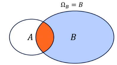
the conditional probability of A given B is $$P_{B}A = P(A \mid B) = \frac{P(A \cap B)}{P(B)}\text{ , for P(B)}> 0.$$

1. $0 \leq P_B(A) \leq 1$ $\because (A \cap B) \subset B \Rightarrow 0 \leq P(A \cap B) \leq P(B) \Rightarrow 0 \leq \frac{P(A \cap B)}{P(B)} \leq 1.$

2. $P_B(B) = 1$ $\because P(B \cap B) = P(B) \Rightarrow \frac{P(B \cap B)}{P(B)} = 1$

3. If $A_1, A_2, \ldots$ are disjoint, then $P_B(\bigcup_{i}A_i) = \sum_{i}P_B(A_i)$ $\frac{P((\bigcup_{i}A_{i}) \cap B)}{P(B)} = \frac{P(\bigcup_{i}(A_{i} \cap B))}{P(B)} = \frac{\sum_{i}P(A_{i} \cap B)}{P(B)} = \sum_{i}\frac{P(A_i \cap B)}{P(B)} = \sum_{i}P(A_{i} \mid B)$

If A and B are independent, $$P(A \mid B) = \frac{P(A)P(B)}{P(B)} = P(A)$$.

2.2.0.1 Multiplicative Rule

Following from the definition of conditional probaility, we have $$P(A \cap B) = P(A \mid B)P(B)$$ For independent events A and B, $P(A\mid B) = P(A) \Rightarrow P(A \cap B) = P(A)P(B).$

Extending to multiple events, $$\begin{align*} P(A \cap B \cap C) &= P(A)\cdot P(B \mid A)\cdot P(C \mid B \cap A) \\ &= P(A \mid B \cap C) \cdot P(B \mid C) \cdot P(C) \end{align*}$$

2.2.0.2 Law of Total Probability

Let $B_1, B_2, \ldots, B_k$ be a partition of sample space $\Omega$.

(i.e. $B_i \cap B_j = \emptyset, \forall i \neq j, and \cup_{i=1}^{k}B_{i} = \Omega.$)

Then for any event A, $$\begin{align*} P(A) &= \sum_{i=1}^{k} P(A \mid B_{i})P(B_{i})\\ &= P(A \cap B_1) + P(A \cap B_2) +\ldots + P(A \cap B_k) \end{align*}$$ i.e. P(A) is the sum of probabilities in each scenario, weighted by each scenario’s probability.

2.2.0.3 Bayes’ Theorem

For $P(B) > 0$, $$P(A \mid B) = \frac{P(B \mid A)\cdot P(A)}{P(B)} = \frac{P(B \mid A)\cdot P(A)}{P(B\mid A)\cdot P(A) + P(B\mid A^c)\cdot P(A^c)}$$

Derivation: By Multiplicative Rule, $$P(A \cap B) = P(A\mid B)\cdot P(B) = P(B\mid A)\cdot P(A)$$ Rearranging, we get Bayes’ Theorem.

2.2.1 Naive Bayes classifier

Applications in supervised learning.

Goal: Classify an input (some object, e.g. an email, image, etc.) into one of several classes using probability.

Let $C$ be a class label (e.g. spam/not spam), and $X = (x_1, x_2, \ldots, x_d)$ be observed features (certain words in the email).

By Bayes’ Theorem, $$P(C \mid X) = \frac{P(X \mid C)P(C)}{P(X)}$$

To find the classifier $\hat{c} := \arg\max_c P(C|X) = \arg\max_c P(X|C)P(C).$

Here, $\arg\max_c P(C \mid X)$ refers to finding the class $c$ that maximises the probability of the class given the data.

This is proportional to $P(X \mid C)P(C)$. We can ignore the denominator $P(X)$, which is a constant for all classes, $C$, during the maximisation process.

From the labelled data, it is easy to find $P(C)$. The challenge is to find $$P(X \mid C) = P(x_1, x_2, \ldots, x_d \mid C).$$

The assumption of Naive Bayes is that all features are conditionally independent, given the class.

Then, we have $$P(x_1, x_2, \ldots, x_d \mid C) = \prod_{i=1}^{d}P(x_i \mid C)$$

The Naive Bayes classifier is now $$\begin{align*} \hat{c} &:= \arg\max_c \prod_{i=1}^{d}P(x_i \mid C)P(C) \\ &:= \arg\max_c P(x_1 \mid C)P(x_2 \mid C)\ldots P(x_d \mid C)P(C) \end{align*}$$

Example calculation of an email spam filter:

From the data, we have $$\begin{gather*} P(\text{spam}) = 0.3, \quad P(\text{not spam}) = 0.7 \\ P(x_1 \mid \text{spam}) = 0.8, \quad P(x_2 \mid \text{spam}) = 0.5, \quad P(x_3 \mid \text{spam}) = 0.3 \\ P(x_1 \mid \text{not spam}) = 0.2, \quad P(x_2 \mid \text{not spam}) = 0.1, \quad P(x_3 \mid \text{not spam}) = 0.2 \end{gather*}$$

Given an input feature {"free", "offer", "click"} $= \{x_1, x_2, x_3\} = \{1, 1, 0\}$,

For class $C$ = spam, $$P(x_1\mid C)P(x_2\mid C)P(x_3\mid C)P(C) = 0.8\cdot0.5\cdot0.7\cdot0.3 = 0.084$$

For class $C$ = not spam, $$P(x_1\mid C)P(x_2\mid C)P(x_3\mid C)P(C) = 0.2\cdot0.1\cdot0.8\cdot0.7 = 0.0112$$

Conclusion: Likely spam.