9 Linear & Logistic Regression

9.1 Types of machine learning

9.1.0.1 Supervised learning

The training data consists of input-output pairs $(x, y)$, where:

• $x$ = the input features

• $y$ = the output label

The goal is to learn the true underlying relationship between $x$ and $y$ from these examples, so that when you see a new, unseen $x$, you can correctly predict its $y$.
The real-life challenge is that the quality of a supervised learning model is heavily dependent on the quality and quantity of labelled data.

9.1.0.2 Unsupervised learning

The training data consists of only inputs $x$ — there are no output labels $y$.
The model must find structure, patterns, or useful knowledge entirely on its own.

9.2 Types of Supervised learning problems

9.2.0.1 Regression

The output $y$ is a continuous value - meaning it can take any real number within some range, rather than belonging to a fixed set of categories.

9.2.0.2 Classification

The output $y$ is a discrete value - meaning it belongs to one of a fixed, finite set of categories or classes.
Both types of problems have different loss functions and model designs.

9.3 Linear Regression

The simplest form of regression problem is linear regression.
For an input data point $x \in \mathbb{R}^d$ (meaning $x$ is a vector of $d$ numbers, i.e. $d$ features), we predict its label $y \in \mathbb{R}$ using $$y \approx w^T x + b$$ where $w \in \mathbb{R}^d$ is the weight vector and each element $w_j$ controls how much the $j$-th feature of $x$ contributes to the prediction. The bias parameter $b \in \mathbb{R}$ shifts the entire prediction up or down regardless of $x$.

9.3.1 Basis functions

A limitation of the basic equation $w^T x + b$ is that it can only represent straight, linear functions.
We introduce basis functions $\phi_j : \mathbb{R}^d \rightarrow \mathbb{R}$ for $j=1, 2, ..., p$. Instead of feeding the raw input $x$ into a linear model, we first transform $x$ using these basis functions, then apply a linear model to the transformed features. $$y \approx w^T \phi(x) + b$$ Note that the model remains linear with respect to its learnable weights ($w$), meaning it is still computationally easy to train. However, it becomes non-linear with respect to the original inputs ($x$), allowing it to fit curved data.

9.3.1.1 Example - polynomial basis functions

If our input is 1D ($d=1$), we can define our basis functions simply as powers of $x$: $\phi_j(x) = x^j$.
Plugging this into the model: $$w^T \phi(x) + b = w_p x^p + w_{p-1} x^{p-1} + ... + w_1 x + b$$

9.4 Parameter Estimation for Linear Regression

Given the linear model and training data, how to find the best possible set of weights?
Here, we assume bias $b=0$.

9.4.1 Least Squares Method (LSM)

Given a dataset of $n$ training examples denoted as $(x_i, y_i)$ for $i = 1, \dots, n$ , LSM attempts to find the optimal weight vector, denoted as $\hat{w}$, by minimizing the average squared difference between the model’s predictions and the actual true labels. $$\hat{w} = \arg \min_{w \in \mathbb{R}^d} \sum_{i=1}^n (y_i - w^T x_i)^2$$ Note that in standard Least Squares, the averaging factor of $1/n$ is conventionally omitted from the formula, though it is usually included in broader concepts like Empirical Risk Minimization.
Why squared error?

• Always non-negative — errors above and below the true value don’t cancel each other out.

• Penalises large errors more heavily.

• Mathematically convenient — the squared function is smooth and differentiable everywhere, making it easy to minimise analytically.

In vector/matrix formulation, if we stack the $n$ labels into a vector $y \in \mathbb{R}^n$, and stack all input features into a matrix $X^T \in \mathbb{R}^{d \times n}$, we get $$\hat{w} = \arg \min_{w \in \mathbb{R}^d} \|y - Xw\|^2$$ Because of this matrix formulation, if we assume that the covariance-like matrix $\hat{\Sigma} = X^T X$ is invertible, we can solve for the optimal weights directly without iterative guessing. The exact, closed-form solution is: $$\hat{w} = \hat{\Sigma}^{-1} X^T y$$ This is derived by taking the gradient of $\|y - Xw\|^2$ with respect to $w$, setting it to zero, and solving. $\hat{\Sigma} = X^TX$ is invertible when the columns of $X$ are linearly independent. This means that $n \geq d$ (i.e. at least as many training examples as features), and no redundant features (i.e. no linear combination of another column).
If $\hat{\Sigma}$ is not invertible, the solution is not unique — multiple values of $w$ give the same minimum loss.

9.4.2 MLE

MLE takes a probabilistic perspective rather than purely looking at geometric errors. It assumes that there is some "true" unknown weight $w_*$ , but the real-world labels we observe ($y$) are corrupted by random Gaussian noise.
Therefore, the rule generating our data is $$y = w_*^T x + \varepsilon, \quad \varepsilon \sim N(0, \sigma^2), \quad y \sim N(w_*^T x, \sigma^2)$$ We want to find the true weights $w_*$.
The probabilistic model of $y$ that is normal distributed, centered at $w_*^T x$, with spread $\sigma^2$ is $$P(y|w,x)=N(w^T x,\sigma^2)(y)$$ Assuming the training examples are independent of each other given their inputs, the joint probability of observing all labels $y = [y_1, ..., y_n]^T$ is: $$\begin{align*} p(y|w,X)&=\prod_{i=1}^n N(w^T x_i, \sigma^2)(y_i)\\ &= \frac{1}{(2\pi\sigma^2)^{n/2}} \prod_{i=1}^n \exp\left(-\frac{1}{2\sigma^2}(y_i - w^T x_i)^2\right) \end{align*}$$ Taking logarithm on both sides, $$\log(p(y|w,X)) = -\frac{n}{2}\log(2\pi\sigma^2) - \sum_{i=1}^n \frac{1}{2\sigma^2}(y_i - w^T x_i)^2$$ The MLE problem is then: $$\hat{w} = \arg \max_{w\in\mathbb{R}^d} \left\{-\frac{n}{2}\log(2\pi\sigma^2) - \sum_{i=1}^n \frac{1}{2\sigma^2}(y_i - w^T x_i)^2\right\}$$ Note that

1. The first term is a constant with respect to $w$ — it doesn’t affect which $w$ is optimal.

2. The second term is a negative scaled version of the LSM objective. Maximising the log-likelihood is exactly equivalent to minimising the sum of squared errors.

Hence, LSM and MLE under Gaussian give the same answer.

9.4.3 Other loss functions (not Gaussian)

The squared error formula $\sum (y_i - w^T x_i)^2$ is entirely attributed to our assumption that the underlying noise is Gaussian.
But what if the data has a different noise structure?
Assume the noise follows a Laplace distribution, defined as $$p(y) = \frac{1}{2b}\exp(-\frac{|y-\mu|}{b})$$ The Laplace distribution has heavier tails — meaning it assigns higher probability to values far from the mean. In practice this means it’s a better model for data with outliers.
Following the same logic as before, the joint likelihood is: $$p(y|w,X)=\frac{1}{(2b)^n}\prod_{i=1}^{n}\exp(-\frac{1}{b}|y_i-w^T x_i|)$$ Maximising the log-likelihood gives: $$\hat{w} = \arg \max_{w \in \mathbb{R}^d} \left\{ -n \log(2b) - \sum_{i=1}^n \frac{1}{b}|y_i - w^T x_i| [cite_start]\right\}$$ Dropping constants, we get $$\hat{w} = \arg \min_{w \in \mathbb{R}^d} \sum_{i=1}^n |y_i - w^T x_i|$$ This simplifies to finding the weights that minimize the absolute error instead of squared error.
The implication is that every choice of loss function corresponds to an implicit assumption about the noise distribution in the data.

9.5 Overfitting & Regularisation

9.5.1 Overfitting

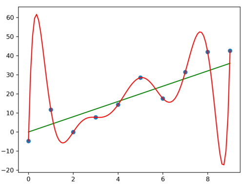
Increasing a model’s complexity (like using higher-degree polynomials) gives it more expressive power. If a model has a higher degree of freedom than the true function that generated the data, it can cause overfitting. In other words, the model learns not just the true underlying pattern in the data, but also the random noise specific to the training set. Graphically, an overfitted curve would try to hit every data point, causing aggressive fluctuations, and making a new prediction on unseen data would be inaccurate.

9.5.2 Ridge regression ($L_2$-Regularisation)

To combat overfitting, we add a regularisation term to the LSM objective. This term penalises large parameter values, discouraging the model from becoming too complex and fitting the noise. $$\hat{w} = \arg \min_{w \in \mathbb{R}^d} \{||y - Xw||^2 + \lambda||w||^2\}$$ The $L_2$ regularisation term $\lambda||w||^2$ consists of:

• $\lambda > 0$, the regularisation strength.

• $\|w\|^2 = w_1^2 + \ldots + w_n^2$, the sum of squares of all the weights.

Recall that overfitting is caused by the model making wild swings between data points, and this requires large weight values.
Hence, the model now has to balance two competing goals:

1. Minimising the squared error, and

2. keeping the weights as small as possible.

Just like standard LSM, Ridge regression has a closed-form solution.
With $\hat{\Sigma} = X^T X$, $$\hat{w} = (\lambda I + \hat{\Sigma})^{-1} X^T y$$ Recall that standard LSM requires $\hat{\Sigma} = X^T X$ to be invertible, which fails when there aren’t enough training examples or features are redundant. Adding $\lambda I$ to $\hat{\Sigma}$ always makes the matrix invertible for any $\lambda > 0$, since it shifts all eigenvalues away from zero. This means Ridge regression is well-defined even when standard LSM breaks down.

9.5.2.1 Effect of regularisation strength $\lambda$

$\lambda$ affects how much to penalise large weights.

1. No regularization ($\lambda = 0$): This is just pure LSM with no penalty on weights, prone to overfitting.

2. Proper regularization ($\lambda$ at the right value): The model is constrained enough to ignore noise but flexible enough to capture the true shape. Strikes a good balance between training fit and generalisation

3. Strong regularization ($\lambda$ very large): The penalty on weight is too high, flattening the curve entirely into a straight line, leading to underfitting

In practice, $\lambda$ might be chosen through cross-validation, i.e. testing different values of $\lambda$ using training set and a validation set. $\lambda$ is a hyperparameter, meaning it’s a parameter of the learning algorithm itself, not learned from the data directly like $w$, but chosen by the user.

9.6 Bias-variance tradeoff

Recall the linear regression model: $$y_i = w_*^T x_i + \varepsilon_i$$ for fixed input data points $x_i$, for $i=1,\ldots,n$.
The noise has mean of 0, variance of $\sigma^2$, and all the $\varepsilon_i$ are independent of each other.
From the training data, we train the model, and get an estimated set of weights. This is the estimator $\hat{w}$, which is a function of the observed labels $y_i$. The implication is that $\hat{w}$ is a random variable.

9.6.1 How good is the estimator $\hat{w}$?

We measure the expected squared error: $$\frac{1}{n} \mathbb{E}[||X(\hat{w} - w_*)||^2]$$ This is the average squared difference between what the model predicts ($X\hat{w}$) and what the true prediction should be ($Xw_*$).
By adding and subtracting $E[\hat{w}]$, we get $$\underbrace{\frac{1}{n} \mathbb{E}[||X(\hat{w} - \mathbb{E}[\hat{w}])||^2]}_{\text{Variance}} \:+\: \underbrace{\frac{1}{n} ||X(\mathbb{E}[\hat{w}] - w_*)||^2}_{\text{Bias squared}}$$ Interpretation:

• Variance term: This measures how much the model’s predictions fluctuate around its own mean due to noise in the underlying data. High variance means that different training datasets give very different $\hat{w}$ values.

• Bias squared term: This measures the difference between the model’s average prediction and the true underlying rule. If $\mathbb{E}[\hat{w}] = w_*$, we get an unbiased estimator.

Connection to overfitting/underfitting:

• A simple model (high regularisation weight $\lambda$) would have high bias (can’t capture the true patterns) and low variance (relatively stable across diff dataset).

• A complex model (low $\lambda$) would have low bias (model is flexible to fit to the data) and high variance (sensitive to noise).

In both cases, the total error is high. The goal is find the sweet spot that minimises their sum by choosing the right regularisation weight $\lambda$.

9.6.2 Performance of Ridge Regression

Recall the formula for Ridge Regression weights (our estimator, $\hat{w}$): $$\hat{w} = (\lambda I + \hat{\Sigma})^{-1} X^T Y, \quad \hat{\Sigma} = X^TX$$ Bias term
Since the true labels are generated by $Y = Xw_* + \varepsilon$, subbing in, $$\begin{align*} \hat{w} &= (\lambda I + \hat{\Sigma})^{-1} X^T (Xw_* + \varepsilon)\\ &= (\lambda I + \hat{\Sigma})^{-1} (\hat{\Sigma} w_* + X^T \varepsilon) \end{align*}$$ Then taking expectation, $$\mathbb{E}[\hat{w}] = (\lambda I + \hat{\Sigma})^{-1}\hat{\Sigma} w_*$$ because $\mathbb{E}[\varepsilon]=0$.
Note that $\mathbb{E}[\varepsilon]\neq w_*$, instead it depends on both $\lambda$ and $\hat{\Sigma}$.
Since the bias is the difference between $\mathbb{E}[\varepsilon]$ and the truth $w_*$, $$\begin{align*} \text{bias squared} &= \frac{1}{n}\|X(\mathbb{E}[\hat{w}] - w_*)\|^2\\ &= \frac{\lambda^2}{n}\|X(\lambda I + \hat{\Sigma})^{-1}w_*\|^2\\ &= \frac{\lambda^2}{n} w_*^T (\lambda I + \hat{\Sigma})^{-2} \hat{\Sigma} w_* \end{align*}$$ Variance term
The variance for Ridge Regression estimator is $$\text{Variance} = \frac{1}{n} E[||X(\hat{w} - E[\hat{w}])||^2] = \frac{\sigma^2}{n} Tr((\lambda I + \hat{\Sigma})^{-2} \hat{\Sigma}^2)$$

Therefore, for Ridge regression with $L_2$-regularisation ($\lambda$), we have: $$\frac{1}{n} \mathbb{E}[||X(\hat{w} - w_*)||^2] = \underbrace{\frac{\lambda^2}{n} w_*^T (\lambda I + \hat{\Sigma})^{-2} \hat{\Sigma} w_*}_{\text{Bias}^2} + \underbrace{\frac{\sigma^2}{n} Tr((\lambda I + \hat{\Sigma})^{-2} \hat{\Sigma}^2)}_{\text{Variance}}$$ Key observations:

• $\lambda=0$ (No regularisation): $\hat{w}$ is the LSM/MLE estimator. Ridge regression reduces to just to standard LSM, which is equivalent to MLE under Gaussian noise.

  • $\text{Bias}^2 = 0$, Variance $= \frac{\sigma^2 d}{n}$, Total error $= \frac{\sigma^2 d}{n}$.

  • This estimator is unbiased. The variance can be large if $d$ is large and $n$ is small (many parameters relative to data).

  • Hence $n>>d$ is required for MLE/LSM to perform well.

  • Prone to overfitting.

• $\lambda\to\infty$ (Strong regularisation): The estimator becomes useless.

  • $\text{Bias}^2 \to \frac{1}{n}\|Xw_*\|^2$, Variance $\to 0$, Total error $\to \frac{1}{n}\|Xw_*\|^2$.

  • To minimise the loss function, $\hat{w}\to 0$, so it predicts near 0 regardless of $x$. The variance is thus near 0.

  • The bias is huge, as the predictions are consistently wrong.

  • Underfitting.

• The role of $n$ and $d$:

  • If $n=1000$, $d=10$, variance $= 0.01\sigma^2$, which is very small so LSM works well.

  • If $n=d$, variance $=\sigma^2$ is large, so LSM doesn’t learn anything useful.

  • If $n<d$, $\hat{\Sigma}=X^TX$ is not invertible so LSM has no unique solution. Ridge regression fixes this as ($\lambda I + \hat{\Sigma}$) is always invertible, but at the cost of introducing bias.

  • Hence ridge regression trades some bias for a variance reduction, giving better total error.

9.6.3 The Bias-Variance Tradeoff Curve

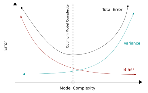
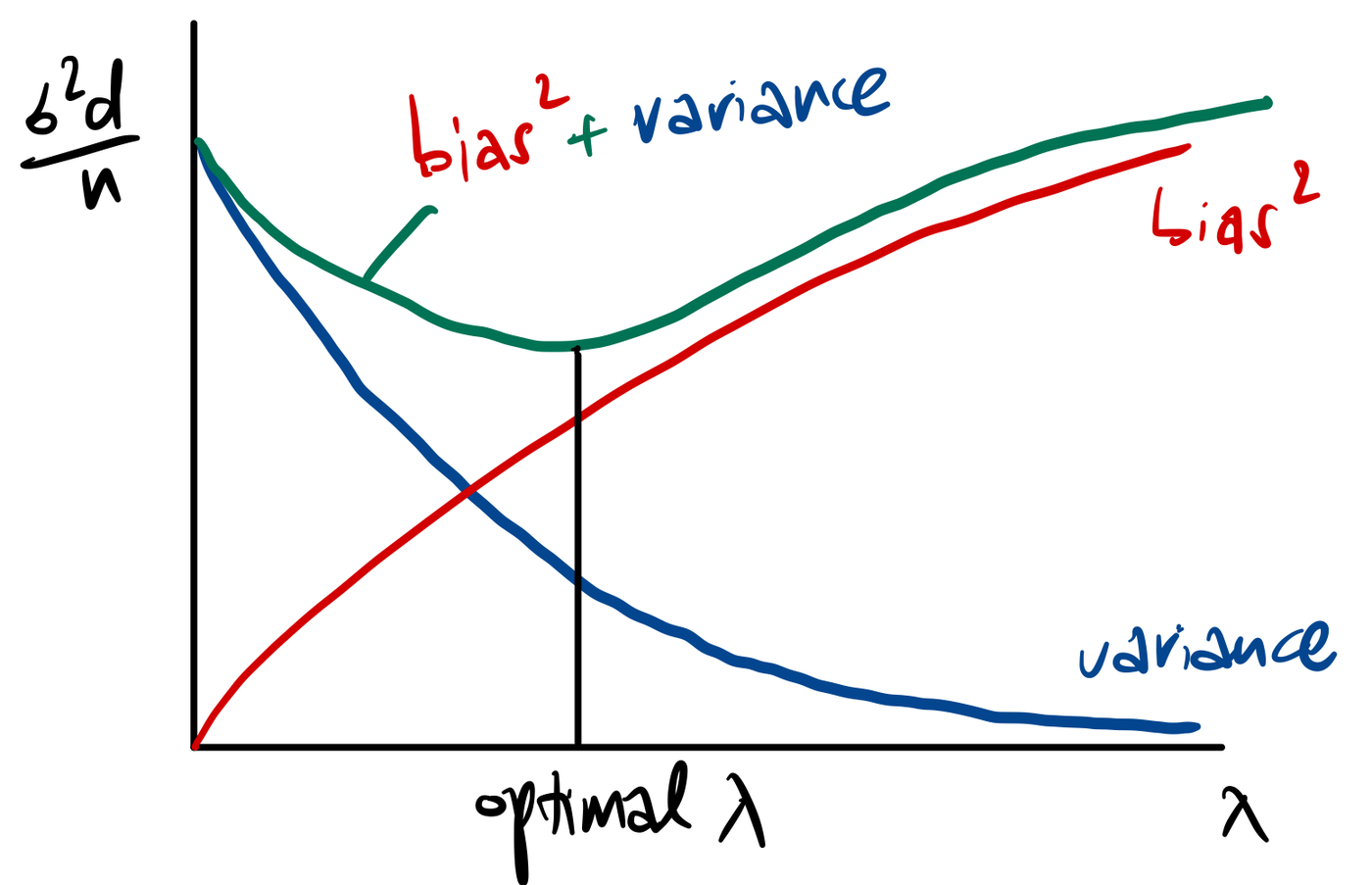
The goal is find $\lambda$ that balances bias (underfitting) and variance (overfitting).

9.7 Logistic Regression

Despite its name, Logistic regression focuses on binary classification problem. We are trying to predict a discrete outcome that only has two possible states, mathematically represented as $y \in \{-1, 1\}$.
We use a sigmoid function to squash a continuous output from the standard linear regression model ($w^T x$), into a valid probability between 0 and 1. The sigmoid function is $$\sigma(z) = \frac{1}{1 + \exp(-z)}$$ Note that:

• When $z$ is large and positive, $\sigma(z)\approx 1/(1+0) = 1$.

• When $z$ is large and negative, $\sigma(z)\approx 1/\infty = 0$.

• When $z=0$, $\sigma(0) = 0.5$.

9.7.0.1 The probabilistic structure

For an input $x \in \mathbb{R}^d$, and an unknown true parameter $w_*\in\mathbb{R}^d$,

• The probability that the class is 1: $\mathbb{P}[Y=+1|x] = \sigma(w_*^T x)$

• The probability that the class is -1: $\mathbb{P}[Y=-1|x] = 1 - \sigma(w_*^T x)$

9.7.0.2 The decision boundary

Note this critical equivalence: $$w_*^T x \ge 0 \Leftrightarrow \sigma(w_*^T x) \ge 0.5$$ Hence when $w^T x > 0$, the probability of $Y = +1$ is $> 50\%$, so we can predict class of +1.
Conversely, when $w^T x < 0$, the probability of $Y = +1$ is $< 50\%$, so we can predict class of -1.
$w^T x = 0$ is the decision boundary. Geometrically, it is a hyperplane in the input space, dividing it into two sides.

9.7.0.3 Unifying the probabilistic structure

Combining the 2 probabiliy equations, $$p(y|x,w) = \frac{1}{1 + \exp(-y w^T x)}$$ We can check that:

• When $y=+1$, $p(+1|x,w) = \frac{1}{1 + \exp(-w^T x)} = \sigma(w^Tx)$.

• When $y=-1$, $p(-1|x,w) = \frac{1}{1 + \exp(w^T x)} = 1 - \sigma(w^Tx)$.

9.7.1 MLE for Logistic Regression

Given training data $(x_i, y_i)$ for $i = 1,\ldots,n$ and assuming the training examples are independent, the MLE objective is to find $$\begin{align*} \hat{w} &= \arg \max_{w \in \mathbb{R}^d} \sum_{i=1}^n \log(p(y_i|x_i,w))\\ &= \arg \max_{w \in \mathbb{R}^d} \sum_{i=1}^n \log \left(\frac{1}{1 + \exp(-y_i w^T x_i)}\right)\\ &= \arg \max_{w \in \mathbb{R}^d} \sum_{i=1}^n -\log (1 + \exp(-y_i w^T x_i))\\ &= \arg \min_{w \in \mathbb{R}^d} \sum_{i=1}^n \log (1 + \exp(-y_i w^T x_i)) \end{align*}$$ Intuition behind this logistic loss:

• When the prediction is correct and confident ($y_i$ and $w^Tx_i$ have the same sign, large magnitude), we get $\approx\log(1+0)=0$, a small loss.

• When the prediction is wrong and confident ($y_i$ and $w^T x_i$ have opposite signs, large magnitude), we get $\log(1+\infty)\to \infty$, a very large loss.

• When the model is uncertain ($w^T x_i \approx 0$), we get $\approx \log(1+1)$, a moderate loss.

To prevent overfitting, we can add $L_2$ regularisation to obtain the final logistic regression objective: $$\hat{w} = \arg \min_{w \in \mathbb{R}^d} \left\{ \frac{1}{n} \sum_{i=1}^n \log(1 + \exp(-y_i w^T x_i)) + \lambda||w||^2 \right\}$$ Probabilistic framework: Logistic regression uses Bernoulli via sigmoid, instead of Gaussian in linear regression.
Closed-form solution: Unlike linear/Ridge regression, logistic regression does not have a closed-form analytical solution. The logistic loss is not quadratic in $w$, so we can’t simply set the gradient to zero and solve algebraically. Instead, iterative numerical methods such as gradient descent must be used to find $\hat{w}$. However, the objective is convex, which guarantees that iterative methods will converge to the global minimum.