3 Random Variables and Distributions

Random variables

A random variable is a function that maps outcomes from a sample space to a real number. X:Ω→ℝX: \Omega \rightarrow \mathbb{R}

Example

Rolling two dice, we have Ω=(i,j)∣i,j∈{1,2,3,4,5,6}\Omega = {(i, j)\mid i,j\in \{1,2,3,4,5,6\}}.

We can define several random variables on Ω\Omega.

  1. Sum: X((i,j))=i+jX((i,j)) = i + j

  2. Larger of the two: X((i,j))=max⁡(i,j)X((i, j)) = \max(i, j)

  3. Indicator of doubles: X(ω)={1if i=j0elseX(\omega) = \begin{cases} 1 & \text{if }i = j \\ 0 & \text{else} \end{cases}

3.0.0.1 Discrete Random Variables

X has a finite or countably infinite range of possible values. Range(X)={n1,n2,…,nk} or {n1,n2,…}\text{Range}(X) = \{n_1, n_2, \ldots, n_k\} \text{ or } \{n_1, n_2, \ldots\}

3.0.0.2 Continuous Random Variables

X takes values in an uncountable subset/interval of ℝ\mathbb{R}. Range(X)⊂ℝ, an interval/continuum\text{Range}(X) \subset \mathbb{R}\text{, an interval/continuum}

Probability law of random variables

For a probability space (Ω,P)(\Omega, P), and random variable X:Ω→ℝX: \Omega \rightarrow \mathbb{R},

and for any set A⊆ℝA \subseteq \mathbb{R}, the probability law/distribution of X is

PX(A)=P(X∈A)=P(X−1(A))=P({ω∈Ω:X(ω)∈A})P_X(A) = P(X\in A) = P(X^{-1}(A)) = P(\{\omega\in\Omega: X(\omega)\in A\})

Instead of discussing PP on Ω\Omega, we look at the push-forward measure of PP by XX, where PX(A)P_X(A) is the likelihood of event A⊆ℝA\subseteq\mathbb{R} occuring.

The corresponding sample space is Ω′=Range(X)={X(ω)∣ω∈Ω}\Omega' = \text{Range}(X) = \{X(\omega)\mid \omega\in\Omega\}.

We say that XX follows the probability distribution PXP_X.

Proof that PXP_X is a valid probability measure:

  1. 0≤PX(A)≤10\leq P_X(A)\leq 1

  2. PX(Ω′)=P(X−1(Ω′))=P(Ω)=1P_X(\Omega') = P(X^{-1}(\Omega')) = P(\Omega) = 1

  3. For A1,A2,…⊂Ω′,Ai∩Aj=∅,i≠jA_1, A_2,\ldots\subset\Omega',\: A_i\cap A_j=\emptyset,\:i\neq j, (disjoint sets)
    PX(∪Ai)=P(X−1(∪Ai))=P(∪X−1(Ai))=∑P(X−1(Ai))=∑PX(Ai)P_X(\cup A_i) = P(X^{-1}(\cup A_{i})) = P(\cup X^{-1}(A_i)) = \sum P(X^{-1}(A_i)) = \sum P_X(A_i)

3.1 Cumulative Distribution Function

The CDF of some discrete/continuous random variable XX is FX(t)=PX({x∣x≤t})=P(X≤t)=P(X∈(−∞,t])F_X(t) = P_X(\{x\mid x\leq t\}) = P(X\leq t) = P(X\in (-\infty,t])

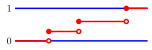
Discrete CDF

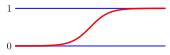
Continuous CDF

Properties:

  1. FX(t)F_X(t) is non-decreasing.

  2. limt→−∞FX(t)=0,limt→+∞FX(t)=1\lim\limits_{t\to -\infty}F_X(t) = 0,\: \lim\limits_{t\to +\infty}F_X(t) = 1

  3. FX(t)F_X(t) is right-continuous (limx→t+F(x)=F(t)\lim\limits_{x\to t^{+}}F(x) = F(t)).

P(X∈(a,b])=FX(b)−FX(a)P(X\in (a, b]) = F_X(b) - F_X(a).

3.2 Probability Mass Function

The PMF of some discrete random variable XX is pX(x)=PX(x)=P(X=x)p_X(x) = P_X({x}) = P(X = x)

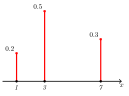
Probability Mass Function

Properties:

  1. pX(x)≥0p_X(x) \geq 0

  2. ∑x∈Range(X)pX(x)=1\sum\limits_{x\in \text{Range}(X)}p_X(x) = 1

  3. FX(x)=∑t≤xpX(t)F_X(x) = \sum\limits_{t\leq x}p_X(t)
    E.g. For the probability that a dice roll is 3 or less, we sum the PMF values for 1, 2, 3.

Referring to the discrete CDF graph, the height of each vertical jump is equal to the probability pX(x)p_X(x) of that specific value.

The CDF FX(x)F_X(x) is right-continuous to ensure that FX(x)=P(X≤x)F_X(x) = P(X \leq x) includes the probability of xx itself (P(X=x)P(X=x)).

Example for number of "heads" in 2 coin flips:

Ω={(H,H),(H,T),(T,H),(T,T)}\Omega = \{(H,H), (H,T), (T,H), (T,T)\},

X(ω)X(\omega) = Number of HH

Ω′=Range(X)={0,1,2}\Omega' = \text{Range}(X) = \{0,1,2\} pX(0)=14,pX(1)=12,pX(2)=14p_X(0) = \frac{1}{4},\:p_X(1) = \frac{1}{2}, \:p_X(2) = \frac{1}{4}

3.2.1 Bernoulli Distribution

A discrete random variable XX with a Bernoulli Distribution takes two values, X∈{0,1}X\in \{0,1\} and with probability mass function P(X=1)=p,P(X=0)=1−pP(X=1) = p,\:P(X=0)=1-p Used to model scenarios with binary outcomes, like Heads or Tails.

3.2.2 Categorical Distribution

A random variable XX with a Categorical Distribution takes one of K-discrete categories, X∈{1,2,…,K}X\in \{1,2,\ldots,K\} and with probability mass function P(X=i)=pi,pi≥0,∑i=1Kpi=1P(X=i) = p_i,\hspace{0.5cm}p_i\geq 0,\hspace{0.5cm} \sum_{i=1}^K p_i=1 It is a multi-class extension of the Bernoulli Distribution. When K=2K=2, it becomes the Bernoulli Distribution.

3.3 Probability Density Function

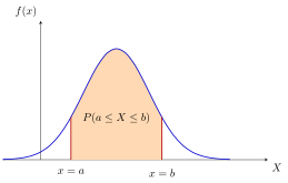
The PDF of some continuous random variable XX is, (given some event A) fX(A)=P(X∈A)=∫AfX(x)dxf_X(A) = P(X\in A) = \int_A f_X(x)\,\mathrm{d}x

P(a≤X≤b)=∫abfX(x)dxP(a\leq X\leq b) = \int_a^b f_X(x)\,\mathrm{d}x

Properties:

  1. fX(x)=ddxFX(x)f_X(x) = \frac{\mathrm{d}}{\mathrm{d}x}F_X(x), when fXf_X is continuous.
    PDF graph is the derivative of CDF graph, and CDF is the integral of the PDF graph.

  2. fX(x)≥0f_X(x) \geq 0

  3. ∫−∞+∞fX(x)dx=1\int_{-\infty}^{+\infty}f_X(x)\mathrm{d}x = 1

  4. FX(x)=PX((−∞,x])=∫−∞xfX(t)dtF_X(x) = P_X((-\infty, x]) = \int_{-\infty}^{x} f_X(t) \, dt

3.4 Gaussian/Normal Distribution

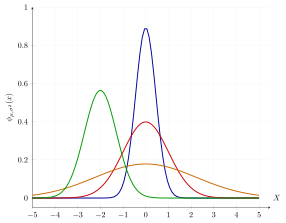
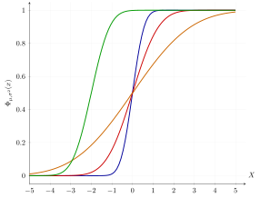
The Gaussian Distribution has a symmetric bell curve shape.

Since it is a continous probability distribution, it can be modelled by a PDF or CDF.

Gaussian/normal distribution N(μ,σ2)N(\mu,\sigma^2) fX(x)=12πσ2exp⁡(−(x−μ)22σ2)f_X(x) = \frac{1}{\sqrt{2\pi\sigma^2}} \exp(-\frac{(x-\mu)^2}{2\sigma^2})

The Standard Gaussian distribution is N(0,1)N(0,1). fX(x)=12πexp⁡(−x22)f_{X}(x)=\frac{1}{\sqrt{2\pi}}\exp(\frac{-x^2}{2})

3.4.0.1 Proportionality (∝\propto)

The constant normalization factors is usually omitted for simplification. A PDF is often written as p(x)=g(x)Z⇒p(x)∝g(x)p(x) = \frac{g(x)}{Z} \Rightarrow p(x) \propto g(x)

By extension, we can identify a Gaussian by Inspection. If a function has the quadratic form in its exponent, it is a Gaussian distribution, even if the constant is missing.
Example: p(x)∝exp⁡(−12σ2x2+μσ2x)p(x) \propto \exp\left( -\frac{1}{2\sigma^2}x^2 + \frac{\mu}{\sigma^2}x \right) By completing the square in the exponent, we can identify this as 𝒩(μ,σ2)\mathcal{N}(\mu, \sigma^2): RHS=exp⁡(−12σ2(x−μ)2)⋅exp⁡(μ22σ2)\text{RHS} = \exp\left( -\frac{1}{2\sigma^2}(x - \mu)^2 \right) \cdot \exp\left( \frac{\mu^2}{2\sigma^2} \right) The term exp⁡(μ22σ2)\exp\left( \frac{\mu^2}{2\sigma^2} \right) is constant with respect to xx and can be absorbed into the proportionality constant.

CDF of normal distribution

3.4.1 Gaussian Integral

To prove that the Gaussian PDF integrates to 1, we use the standard Gaussian integral result: ∫−∞∞e−x2dx=π\int_{-\infty}^{\infty} e^{-x^2} \, dx = \sqrt{\pi} By applying the change of variable y=12σ2(x−μ)y = \frac{1}{\sqrt{2\sigma^2}}(x - \mu), we can derive: ∫−∞∞exp⁡(−12σ2(x−μ)2)dx=2πσ2\int_{-\infty}^{\infty} \exp\left( -\frac{1}{2\sigma^2}(x - \mu)^2 \right) \, dx = \sqrt{2\pi\sigma^2} The general form of the Gaussian integral is ∫−∞∞e−ax2dx=πa\int_{-\infty}^{\infty} e^{-ax^2} \, dx = \sqrt{\frac{\pi}{a}}

3.5 Bayesian Inference

Example

3.5.1 The Goal

We wish to find the posterior distribution P(μ∣x1,…,xn)P(\mu \mid x_1, \dots, x_n), which represents our updated belief about the mean μ\mu after observing the data.

Bayes’ Rule Formulation

Using Bayes’ Rule, the posterior is proportional to the likelihood times the prior: P(μ∣x1,…,xn)=P(x1,…,xn∣μ)P(μ)P(x1,…,xn)P(\mu \mid x_1, \dots, x_n) = \frac{P(x_1, \dots, x_n \mid \mu) P(\mu)}{P(x_1, \dots, x_n)} Since the denominator P(x1,…,xn)P(x_1, \dots, x_n) does not depend on μ\mu, we treat it as a normalization constant and write: P(μ∣x1,…,xn)∝P(x1,…,xn∣μ)⋅P(μ)P(\mu \mid x_1, \dots, x_n) \propto P(x_1, \dots, x_n \mid \mu) \cdot P(\mu)

Defining the Components

1. The Likelihood Function
Since the samples are independent, the joint probability is the product of individual probabilities: P(x1,…,xn∣μ)=∏i=1nP(xi∣μ)=∏i=1n12πσ2exp⁡(−12σ2(xi−μ)2)∝exp⁡(−12σ2∑i=1n(xi−μ)2)\begin{align*} P(x_1, \dots, x_n \mid \mu) &= \prod_{i=1}^{n} P(x_i \mid \mu) \\ &= \prod_{i=1}^{n} \frac{1}{\sqrt{2\pi\sigma^2}} \exp\left( -\frac{1}{2\sigma^2}(x_i - \mu)^2 \right) \\ &\propto \exp\left( -\frac{1}{2\sigma^2} \sum_{i=1}^{n} (x_i - \mu)^2 \right) \end{align*}

. The Prior Function
Our prior belief is a single Gaussian centered at μ0\mu_0: P(μ)=12πσ02exp⁡(−12σ02(μ−μ0)2)∝exp⁡(−12σ02(μ−μ0)2)\begin{align*} P(\mu) &= \frac{1}{\sqrt{2\pi\sigma_0^2}} \exp\left( -\frac{1}{2\sigma_0^2}(\mu - \mu_0)^2 \right) \\ &\propto \exp\left( -\frac{1}{2\sigma_0^2}(\mu - \mu_0)^2 \right) \end{align*}

The Combined Equation

Multiplying the Likelihood and Prior (by adding their exponents): P(μ|data)∝exp⁡([−12σ2∑i=1n(xi−μ)2]+[−12σ02(μ−μ0)2])P(\mu | \text{data}) \propto \exp\left( \left[ -\frac{1}{2\sigma^2} \sum_{i=1}^{n} (x_i - \mu)^2 \right] + \left[ -\frac{1}{2\sigma_0^2}(\mu - \mu_0)^2 \right] \right)

3.5.2 The math

Expanding the Squares

We expand the quadratic terms. Note that any term not containing μ\mu is effectively a constant relative to μ\mu and can be absorbed into the proportionality constant. ∑i=1n(xi−μ)2=∑xi2−2μ∑xi+nμ2(μ−μ0)2=μ2−2μμ0+μ02\begin{align*} \sum_{i=1}^{n}(x_i - \mu)^2 &= \sum x_i^2 - 2\mu\sum x_i + n\mu^2 \\ (\mu - \mu_0)^2 &= \mu^2 - 2\mu\mu_0 + \mu_0^2 \end{align*} Discarding terms without μ\mu (like ∑xi2\sum x_i^2 and μ02\mu_0^2), the relevant part of the exponent is: −12[nμ2−2μ∑xiσ2+μ2−2μμ0σ02]-\frac{1}{2} \left[ \frac{n\mu^2 - 2\mu\sum x_i}{\sigma^2} + \frac{\mu^2 - 2\mu\mu_0}{\sigma_0^2} \right]

Grouping Coefficients

We group the terms by μ2\mu^2 and μ\mu: −12[μ2(nσ2+1σ02)−2μ(∑xiσ2+μ0σ02)]-\frac{1}{2} \left[ \mu^2 \left( \frac{n}{\sigma^2} + \frac{1}{\sigma_0^2} \right) - 2\mu \left( \frac{\sum x_i}{\sigma^2} + \frac{\mu_0}{\sigma_0^2} \right) \right] This matches the standard Gaussian form −12σnew2(μ−μnew)2-\frac{1}{2\sigma_{new}^2}(\mu - \mu_{new})^2, which expands to −12σnew2(μ2−2μμnew)-\frac{1}{2\sigma_{new}^2}(\mu^2 - 2\mu\mu_{new}).

3.5.3 The posterior parameters

By comparing coefficients, we derive the Posterior Variance (σn2\sigma_n^2) and Mean (μn\mu_n):

Posterior Variance (σn2\sigma_n^2): 1σn2=nσ2+1σ02⇒σn2=σ2σ02nσ02+σ2\frac{1}{\sigma_n^2} = \frac{n}{\sigma^2} + \frac{1}{\sigma_0^2} \quad \Rightarrow \quad \sigma_n^2 = \frac{\sigma^2 \sigma_0^2}{n\sigma_0^2 + \sigma^2}

Posterior Mean (μn\mu_n): μnσn2=∑xiσ2+μ0σ02⇒μn=σn2(∑xiσ2+μ0σ02)\frac{\mu_n}{\sigma_n^2} = \frac{\sum x_i}{\sigma^2} + \frac{\mu_0}{\sigma_0^2} \quad \Rightarrow \quad \mu_n = \sigma_n^2 \left( \frac{\sum x_i}{\sigma^2} + \frac{\mu_0}{\sigma_0^2} \right)

Numerical Calculation

We apply the values from the problem:

Calculate Variance: σn2=1⋅43(4)+1=413≈0.308\begin{equation*} \sigma_n^2 = \frac{1 \cdot 4}{3(4) + 1} = \frac{4}{13} \approx 0.308 \end{equation*}

Calculate Mean: μn=413(3031+1004)=413(303+25)=413(328)=131213≈100.92\begin{equation*} \mu_n = \frac{4}{13} \left( \frac{303}{1} + \frac{100}{4} \right) = \frac{4}{13} (303 + 25) = \frac{4}{13}(328) = \frac{1312}{13} \approx 100.92 \end{equation*}

Conclusion: The posterior distribution is μ∼𝒩(100.92,0.308)\mu \sim \mathcal{N}(100.92, 0.308).

3.5.4 Interpretationss

The formulas: Variance:σ̂n2=σ2σ02nσ02+σ2Mean:μ̂n=σ̂n2(∑xiσ2+μ0σ02)\begin{align*} \text{Variance:} \quad \hat{\sigma}_n^2 &= \frac{\sigma^2 \sigma_0^2}{n\sigma_0^2 + \sigma^2} \\ \text{Mean:} \quad \hat{\mu}_n &= \hat{\sigma}_n^2 \left( \frac{\sum x_i}{\sigma^2} + \frac{\mu_0}{\sigma_0^2} \right) \end{align*}

1. Prior unconfidence (σ02→∞\sigma_0^2 \to \infty)

Imagine we have zero confidence in our prior belief (variance is infinite).

Limit of the Variance: limσ02→∞σ̂n2=σ2n\begin{equation*} \lim_{\sigma_0^2 \to \infty} \hat{\sigma}_n^2 = \frac{\sigma^2}{n} \end{equation*}

Limit of the Mean: limσ02→∞μ̂n=σ2n(∑xiσ2+0)=1n∑i=1nxi=x‾\begin{equation*} \lim_{\sigma_0^2 \to \infty} \hat{\mu}_n = \frac{\sigma^2}{n} \left( \frac{\sum x_i}{\sigma^2} + 0 \right) = \frac{1}{n} \sum_{i=1}^{n} x_i = \bar{x} \end{equation*}

Interpretation: This recovers the Frequentist Result. Without a prior, our best guess is simply the sample mean (x‾\bar{x}) and the standard error depends purely on the data variance.

2. Infinite Data (n→∞n \to \infty)

Imagine we collect a massive amount of data.

Limit of the Variance: limn→∞σ̂n2=limn→∞σ2σ02nσ02+σ2=0\begin{equation*} \lim_{n \to \infty} \hat{\sigma}_n^2 = \lim_{n \to \infty} \frac{\sigma^2 \sigma_0^2}{n\sigma_0^2 + \sigma^2} = 0 \end{equation*} (Our uncertainty shrinks to zero; we become perfectly confident).

Limit of the Mean: limn→∞μ̂n=limn→∞σ̂n2(∑i=1nxiσ2+μ0σ02)=limn→∞(σ2σ02nσ02+σ2)nx‾σ2+(σ2σ02nσ02+σ2)μ0σ02=limn→∞σ02x‾σ02+σ2n+0=x‾\begin{align*} \lim_{n \to \infty} \hat{\mu}_n &= \lim_{n \to \infty} \hat{\sigma}_n^2 \left( \frac{\sum_{i=1}^n x_i}{\sigma^2} + \frac{\mu_0}{\sigma_0^2} \right) \\ &= \lim_{n \to \infty} \left( \frac{\sigma^2 \sigma_0^2}{n\sigma_0^2 + \sigma^2} \right) \frac{n\bar{x}}{\sigma^2} + \left( \frac{\sigma^2 \sigma_0^2}{n\sigma_0^2 + \sigma^2} \right) \frac{\mu_0}{\sigma_0^2} \\ &= \lim_{n \to \infty} \frac{\sigma_0^2 \bar{x}}{\sigma_0^2 + \frac{\sigma^2}{n}} + 0 \\ &= \bar{x} \end{align*} (The estimate converges to the true empirical average).

3.5.5 The core philosophy of Bayesian Inference

The prior distribution compensates for the lack of data when the sample size is small.

3.6 Multivariate Random Variables

We now consider two random variables, XX and YY, and assign probability to Z=(X,Y)Z=(X,Y).

For any set A∈ℝ2A\in\mathbb{R}^2, P(X,Y)(A)=P((X,Y)∈A)=P((X,Y)−1A)=P({ω∈Ω:(X(ω),Y(ω))∈A})P_{(X,Y)}(A) = P((X,Y)\in A) = P((X,Y)^{-1}A) = P(\{\omega\in\Omega:(X(\omega),Y(\omega))\in A\}) This is a joint distribution on X,YX,Y.

3.6.1 Cumulative Distributive Function

For two random variables X,YX,Y, their CDF is FX,Y(x,y)=P(X≤x,Y≤y)=P(X∈(−∞,x],Y∈(−∞,y])F_{X,Y}(x,y) = P(X\leq x,Y\leq y) = P(X\in (-\infty,x],Y\in(-\infty,y]) FX,Y:ℝ2→ℝF_{X,Y}: \mathbb{R}^2 \rightarrow \mathbb{R}

3.6.2 Joint Distribution/PMF (Discrete)

For two random variables X,YX,Y, their joint PMF is pX,Y(x,y)=PX,Y({x,y})=P(X=x,Y=y)p_{X,Y}(x,y) = P_{X,Y}(\{x,y\}) = P(X=x, Y=y)

Properties:

  1. pX,Y(x,y)≥0p_{X,Y}(x,y) \geq 0

  2. ∑(x,y)∈Range(X,Y)pX,Y(x,y)=1\sum\limits_{(x,y)\in\text{Range}(X,Y)}p_{X,Y}(x,y) = 1

3.6.3 Marginal Distribution/PMF (Discrete)

Given the joint PMF pX,Y(x,y)p_{X,Y}(x,y), the marginal distributions/PMFs of XX and YY are found by summing over all possible values of the other variable. pX(x)=∑ypX,Y(x,y)p_X(x) = \sum\limits_{y}p_{X,Y}(x,y) pY(y)=∑xpX,Y(x,y)p_Y(y) = \sum\limits_{x}p_{X,Y}(x,y)

𝒀=𝟎\mathbf{Y=0} 𝒀=𝟏\mathbf{Y=1}
𝑿=𝟎\mathbf{X=0} 1/101/10 2/102/10 3/103/10
𝑿=𝟏\mathbf{X=1} 3/103/10 4/104/10 7/107/10
4/104/10 6/106/10 11

The marginal distributions are found in the margins of the table.

3.6.4 Conditional Distribution/PMF (Discrete)

For discrete random variables X,YX,Y and P(Y=y)>0P(Y=y) > 0, PX∣Y(x∣y)=P(X=x∣Y=y)=P(X=x,Y=y)P(Y=y)P_{X\mid Y}(x\mid y) = P(X=x\mid Y=y) = \frac{P(X=x, Y=y)}{P(Y=y)} The probability of X=xX=x given Y=yY=y.

Multiplicative Rule: P(X=x,Y=y)=P(X=x∣Y=y)⋅P(Y=y)P(X=x, Y=y) = P(X=x\mid Y=y)\cdot P(Y=y) The Joint Probability is the product of the Marginal and the Conditional.

3.6.5 Example (Sampling Without Replacement)

Box contains 3 white and 3 black balls. Draw 2 balls without replacement.
X=X = result of first draw (1=1 = white, 0=0 = black)
Y=Y = result of second draw (1=1 = white, 0=0 = black)

PMF: P(X=0,Y=0)=36×25=15,P(X=1,Y=1)=15P(X=0,Y=1)=36×35=310,P(X=1,Y=0)=310\begin{align*} P(X = 0, Y = 0) &= \frac{3}{6} \times \frac{2}{5} = \frac{1}{5}, & P(X = 1, Y = 1) &= \frac{1}{5} \\ P(X = 0, Y = 1) &= \frac{3}{6} \times \frac{3}{5} = \frac{3}{10}, & P(X = 1, Y = 0) &= \frac{3}{10} \end{align*}

Marginals: P(X=1)=12,P(Y=1)=12\begin{equation*} P(X = 1) = \frac{1}{2}, \quad P(Y = 1) = \frac{1}{2} \end{equation*}

We can conclude XX and YY are not independent.

Conditionals:

Since P(X=1,Y=1)=15P(X = 1, Y = 1) = \frac{1}{5} and P(Y=1)=12P(Y = 1) = \frac{1}{2}, the conditional distribution is: P(X=1∣Y=1)=25<12=P(X=1)\begin{equation*} P(X = 1 \mid Y = 1) = \frac{2}{5} < \frac{1}{2} = P(X=1) \end{equation*}

Knowing the second ball is white makes the first less likely to be white.

3.6.6 Joint Distribution/PDF (Continuous)

For continuous random variables X,YX,Y and A⊂ℝ2A\subset \mathbb{R}^2, P((X,Y)∈A)=∬AfX,Y(x,y)dxdyP((X,Y)\in A) = \iint_A f_{X,Y}(x,y)\:\mathrm{d}x\:\mathrm{d}y where fX,Y(x,y)f_{X,Y}(x,y) is the joint PDF.

Properties:

  1. fX,Y(x,y)≥0f_{X,Y}(x,y)\geq 0

  2. ∬ℝ2fX,Y(x,y)dxdy=1\iint_{\mathbb{R}^2}f_{X,Y}(x,y)\:\mathrm{d}x\:\mathrm{d}y = 1

3.6.7 Marginal Distribution/PDF (Continuous)

Given the joint PDF fX,Y(x,y)f_{X,Y}(x,y), the marginal distributions/PDFs of XX and YY are found by integrating out the other variable. fX(x)=∫−∞+∞fX,Y(x,y)dyf_X(x) = \int_{-\infty}^{+\infty}f_{X,Y}(x,y)\:\mathrm{d}y fY(y)=∫−∞+∞fX,Y(x,y)dxf_Y(y) = \int_{-\infty}^{+\infty}f_{X,Y}(x,y)\:\mathrm{d}x

Properties:

  1. fX(x)≥0f_X(x) \geq 0

  2. ∫−∞+∞fX(x)dx=1\int_{-\infty}^{+\infty}f_X(x)\:\mathrm{d}x = 1

3.6.8 Conditional Distribution/PDF (Continuous)

For continuous random variables X,YX,Y and fY(y)>0f_Y(y) > 0, fX∣Y(x∣y)=fX,Y(x,y)fY(y)f_{X\mid Y}(x\mid y) = \frac{f_{X,Y}(x,y)}{f_Y(y)}

Multiplicative Rule: fX,Y(x,y)=fX∣Y(x∣y)fY(y)f_{X,Y}(x,y) = f_{X\mid Y}(x\mid y)f_Y(y)

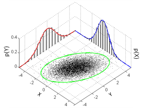
Empirical Scatter Plot
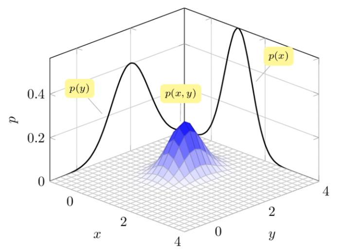
Theoretical PDF Surface
Comparison of Joint Probability Representations

Geometrically, the conditional PDF fY|X(y|x)f_{Y|X}(y|x) is obtained by taking a cross-sectional slice of the joint density surface at a fixed X=xX=x, then normalizing the resulting 1D curve to ensure its area integrates to one.

3.7 Independence of Random Variables

Two random variables X,YX,Y are independent if, for event sets A,BA,B, P(X∈A,Y∈B)=P(X∈A)⋅P(Y∈B)⇔PX,Y(A×B)=PX(A)⋅PY(B)P(X\in A,Y\in B) = P(X\in A)\cdot P(Y\in B) \iff P_{X,Y}(A \times B) = P_X(A)\cdot P_Y(B)

Discrete Case: A⟂B⇔pX,Yx,y=pX(x)pY(y)A\perp B \iff p_{X,Y}{x,y} = p_X(x)p_Y(y)

Continuous Case: A⟂B⇔fX,Yx,y=fX(x)fY(y)A\perp B \iff f_{X,Y}{x,y} = f_X(x)f_Y(y)

Conditional PMF and PDF: pX∣Y(x∣y)=pX(x)p_{X\mid Y}(x\mid y) = p_X(x) and fX,Y(x,y)=fX(x)f_{X,Y}(x,y) = f_X(x)