6 Concentration Inequalities

6.1 Markov’s Inequality

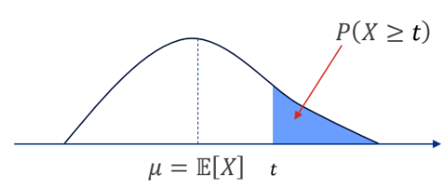
For a non-negative (discrete or continuous) random variable $X$, and $t > 0$, $$P(X \geq t) \leq \frac{\mathbb{E}[X]}{t}$$

Proof. $$\begin{align*} \mathbb{E}[X] &= \int_0^{\infty}xf_X(x)\:\mathrm{d}x \\ &= \int_0^{t}xf_X(x)\mathrm{d}x + \int_t^{\infty}xf_X(x)\:\mathrm{d}x && [\text{split integral at }t]\\ &\geq \int_t^{\infty}xf_X(x)\:\mathrm{d}x && [\because k\geq 0,\: \mathbf{x\geq 0},\: f_X(x)\geq 0]\\ &\geq \int_t^{\infty}kf_X(x)\:\mathrm{d}x && [\text{because x }\geq \text{ t in the integral}]\\ &= t\int_t^{\infty}f_X(x)\mathrm{d}x \\ &= t\cdot P(X\geq t) \end{align*}$$

$\mathbf{X}$ must be non-negative - Counterexample

Let $X$ be a discrete random variable such that $$X = \begin{cases} 100 & \text{with probability } 0.5 \\ -100 & \text{with probability } 0.5 \end{cases}$$

EV is $$\begin{align*} \mathbb{E}[X] &= \sum x \cdot P(X=x) \\ &= (100 \cdot 0.5) + (-100 \cdot 0.5) \\ &= 50 - 50 \\ &= 0 \end{align*}$$

Let $t = 50$. Using Markov’s inequality,

$$P(X\geq 50) \leq \frac{\mathbb{E}[X]}{50}$$ $$\text{LHS} = P(X\geq 50) = P(X = 100) = 0.5$$ $$\text{RHS} = \frac{\mathbb{E}[X]}{t} = \frac{0}{50} = 0$$ Hence, we get a contradiction ($0.5 \leq 0$).
Takeaway: Negative numbers can skew the mean, making it aritficially small.

6.2 Chebyshev’s Inequality

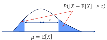
For any random variable $X$, and $t > 0$, $$P \Bigl( |X-\mathbb{E}[X]| \geq t \Bigr) \leq \frac{\mathbb{V}[X]}{t^2}$$

Proof. $$\begin{align*} P \Bigl( |X - \mathbb{E}[X]| \geq t \Bigr) &= P\Bigl((X - \mathbb{E}[X])^2 \geq t^2 \Bigr) && [\because t>0] \\ &\leq \frac{\mathbb{E}[(X - \mathbb{E}[X])^2]}{t^2} && [\text{Markov's Inequality}] \\ &= \frac{\mathbb{V}[X]}{t^2} \end{align*}$$

6.2.1 Alternative form

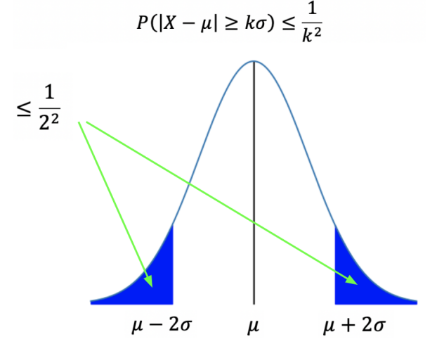
Let $t = k\sigma$, $k > 0$, $\sigma = \sqrt{\mathbb{V}[X]}$. $$P \Bigl( |X-\mathbb{E}[X]| \geq k\sigma \Bigr) \leq \frac{\sigma^2}{(k\sigma)^2} = \frac{1}{k^2}$$ With $k=2$, $\frac{1}{k^2} = \frac{1}{4}$, meaning 75% of data is within 2 standard deviations from the mean.

6.2.2 Markov vs Chebyshev’s inequality

• Values of $\mathbf{X}$: For Markovs’s, $X$ only takes non-negative values, while in Chebyshev’s $X$ can take any value (Squaring the distance from the mean term removes negative values). Markov’s is concerned with position of $X$, while Chebyshev’s cares more about distance from the mean.

• Distribution: Markov’s only requires $\mathbb{E}[X]$, Chebyshev’s requires $\mathbb{E}[X]$ and $\mathbb{V}[X]$.

• Results: Chebyshev’s gives a better estimate than Markov’s.
  Consider a factory producing light bulbs, with $\mathbb{E}[X]=1000$, $\mathbb{V}[X]=2500$. We want to find $P(X \geq 2000)$.
  Markov’s Inequality: $$P(X \geq 2000) \leq \frac{\mathbb{E}[X]}{2000} = \frac{1000}{2000} = 0.5$$ Chebyshev’s Inequality: $$P\Bigl(|X-1000| \geq 1000 \Bigr) \leq \frac{\mathbb{V}[X]}{t^2} = \frac{2500}{1000^2} = 0.0025$$

6.3 (Weak) Law of large numbers

Suppose $X_1, X_2, \ldots, X_n$ are independent and identically distributed (iid) random variables, $$\mathbb{E}[X_i] = \mu,\quad \mathbb{V}[X_i] = \sigma^2,\quad \text{for } i = 1,\ldots,n$$ The empirical average of outcomes is $$\overline{X}_n = \frac{1}{n}\sum_{i=1}^n X_i$$ Then $$\mathbb{E}[\overline{X}_n] = \mu, \quad \mathbb{V}[\overline{X}_n] = \frac{n\sigma^2}{n^2} = \frac{\sigma^2}{n}$$ [Variance decreases as we get more samples ($n \to \infty$)].
Using Chebyshev’s inequality, and for any $\epsilon > 0$, $$P \Bigl(|\overline{X}_n - \mu| \geq \epsilon \Bigr) \leq \frac{\frac{\sigma^2}{n}}{\epsilon^2} = \frac{\sigma^2}{n\epsilon^2}$$ $$\lim\limits_{n \to \infty} P \Bigl(|\overline{X}_n - \mu| \geq \epsilon \Bigr) \leq 0$$ Since probability cannot be less than 0, $$\lim\limits_{n \to \infty} P \Bigl(|\overline{X}_n - \mu| \geq \epsilon \Bigr) \leq 0$$ or $$\lim\limits_{n \to \infty} P \Bigl(|\overline{X}_n - \mu| < \epsilon \Bigr) = 1$$ Interpretation: For a large number $n$, the calculated average $\overline{X}_n$ converges to $\mu$ with absolute certainty. This is because the variance decreases with increasing number of samples.

6.4 Hoeffding’s Inequality

For independent random variables $X_1, \ldots, X_n$, with $a_i \leq X_i \leq b_i$, then $$P \Bigl(|\overline{X}_n - \mathbb{E}[\overline{X}_n]| \geq t \Bigr) \leq 2\exp \left(-\frac{2n^2t^2}{\sum_{i=1}^n(b_i - a_i)^2}\right)$$ Note:

• As the sample size $n$ or error margin $t$ increase, the negative exponent gets more negative, probability $\rightarrow$ 0.

• If the bounds ($b_i - a_i$) are small, the negative exponent gets more negative, probability $\rightarrow$ 0.

Because of the exponenet term, Hoeffding’s inequality gives a tighter bound than Chebyshev’s inequality. $$(\text{Chebyshev's}) \quad O(\frac{1}{nt^2}) \quad \gg \quad \exp(-O(nt^2)) \quad (\text{Hoeffding's})$$ (assuming independence of variables).

6.4.0.1 Example

For iid random variables $X_1,\ldots,X_n$ following Bernoulli distribution, $p = 0.5$,

(Chebyshev’s) $\mathbb{E}[\overline{X}_n] = 0.5,\: \mathbb{V}[\overline{X}_n] = \frac{\mathbb{V}[X]}{n} = \frac{p(1-p)}{n} = \frac{1}{4n}$, $$P\Bigl(|\overline{X}_n - \mathbb{E}[\overline{X}_n]|\geq t \Bigr) \leq \frac{\mathbb{V}[\overline{X}_n]}{t^2} = \frac{1}{4nt^2}$$

(Hoeffding’s) $0\leq X_i \leq 1 \Rightarrow \sum_{i=1}^n(b_i - a_i)^2 = n$, $$P\Bigl(|\overline{X}_n - \mathbb{E}[\overline{X}_n]| \geq t\Bigr) \leq 2\exp\left(-\frac{2n^2t^2}{n}\right) = 2\exp(-2nt^2)$$

6.4.1 Markov v Chebyshev v Hoeffding

6.5 Central Limit Theorem

For a random variable $X$ with mean $\mu$ and standard deviation $\sigma$, the standardisation of $X$ is the new random variable $$Z = \frac{X - \mu}{\sigma}$$ Note that $Z$ has mean 0 and standard deviation 1. Note also that if $X$ has a Gaussian distribution, then the distribution of $X$ is the standard Gaussian distribution $Z$.

Suppose iid random variables $X_1, \ldots, X_n$ each with mean $\mathbb{E}[X]=\mu$ and $\mathbb{V}[X]=\sigma^2$. 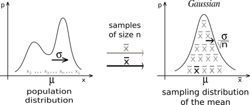Let $\overline{X}_n$ be the average such that $$\overline{X}_n = \frac{X_1 + \ldots + X_n}{n} = \frac{\sum_{i=1}^nX_i}{n}$$ The mean and variance are $$\mathbb{E}[\overline{X}_n] = \mu,\quad \mathbb{V}[\overline{X}_n] = \frac{\sigma^2}{n},\quad \sigma_{\overline{X}_n} = \frac{\sigma}{\sqrt{n}}$$ We can then standardise $\overline{X}_n$ $$Z_n = \frac{\overline{X}_n - \mu}{\sigma / \sqrt{n}}$$ By the Central Limit Theorem, $$\lim\limits_{n\to\infty}P(Z_n \leq t) = \lim\limits_{n\to\infty}P(\frac{\sqrt{n}(\overline{X}_n - \mu)}{\sigma}\leq t) = \frac{1}{\sqrt{2\pi}}\int_{-\infty}^t \exp(-\frac{u^2}{2})\:\mathrm{d}u = \Phi(t)$$ This means that for large $n$, $Z_n$ converges in distribution to the standard Gaussian distribution, and the probability that $Z_n \leq t$ is just the area under the standard Gaussian PDF, from $-\infty \to t$. So as $n \to \infty$, $$\overline{X}_n \sim N(\mu, \frac{\sigma^2}{n}), \quad Z_n \sim N(0, 1)$$

6.5.1 Application of CLT - Normal approximation to binomial

Recall that for a Binomial random variable $X \sim B(n, p)$, $$P(X=k) = \binom{n}{k} p^k (1-p)^{n-k}$$ The problem is that computing this exact probability becomes extremely hard when $n$ and $k$ are large. The factorials inside the $\binom{n}{k}$ term grow massively.
Instead, we can see the Binomial variable as a sum of individual Bernoulli trials.
We define the total successes as $S_n = \sum_{i=1}^n X_i$, where each individual trial $X_i \in \{0, 1\}$.
For each individual Bernoulli trial: $$\mathbb{E}[X_i] = p,\quad \mathbb{V}[X_i] = p(1 - p)$$ Because $S_n$ is a sum of independent trials, we can apply the CLT. By standardising this sum, the distribution becomes approximately normal, as $n \to \infty$, $$\frac{S_n - np}{\sqrt{np(1-p)}} \approx \mathcal{N}(0, 1)$$ We can find the probability that number of successes falls within some lower and upper bounds. $$\begin{align*} P(k \le S_n \le k') &= P\left(\frac{k - np}{\sqrt{np(1-p)}} \le \frac{S_n - np}{\sqrt{np(1-p)}} \le \frac{k' - np}{\sqrt{np(1-p)}}\right) \\ \\ &\approx P\left(\frac{k - np}{\sqrt{np(1-p)}} \le Z \le \frac{k' - np}{\sqrt{np(1-p)}}\right) \quad \text{where } Z \sim \mathcal{N}(0, 1) \\ \\ &= \Phi\left(\frac{k' - np}{\sqrt{np(1-p)}}\right) - \Phi\left(\frac{k - np}{\sqrt{np(1-p)}}\right) \end{align*}$$ Example Flipping a fair coin $n = 40000$ times, what is the probability of getting between 19,600 and 20,400 heads?
Here, computing the exact binomial PMF is not feasible. We use the normal approximation.
Let $S_n$ be the total number of heads. For a fair coin, the probability of heads is $p = 0.5$. $$S_n \sim B(40000, 0.5)$$ Calculating the mean and s.d. for each trial:

• $\mathbb{E}[S_n] = np = 40,000 \times 0.5 = 20,000$

• $\sigma = \sqrt{Var(S_n)} = \sqrt{np(1-p)} = \sqrt{40,000 \times 0.5 \times 0.5} = \sqrt{10,000} = 100$

Thus, we have $$S_n \approx \mathcal{N}(20000, 100^2)$$ Solving, $$\begin{align*} P(19600 \le S_n \le 20400) &= P\left(\frac{19600 - 20000}{100} \le \frac{S_n - 20000}{100} \le \frac{20400 - 20000}{100}\right) \\ \\ &\approx P(-4 \le Z \le 4) \quad \text{where } Z \sim \mathcal{N}(0, 1) \\ &= \Phi(4) - \Phi(-4) \\ &\approx 1 - 0 \approx 0.9999 \end{align*}$$

Example A factory produces items with a defective probability $p$. If we inspect $n$ items, what is the probability regarding the number of defective items?
Let $S_n$ be the total number of defective items in the sample size of $n$, then apply the equation above.

Example If an advertisement has a click through rate of $p$, and the website gets $n$ unique visitors a day, what is the probability regarding the number of clicks?
Let $S_n$ be the total number of ad clicks in the sample size of $n$ visitors, then apply the equation above.