8 Estimation II

8.1 Multimodality

To build generative AI, we rely on Maximum Likelihood Estimation (MLE). However, MLE has a prerequisite: you must first define the mathematical shape of the probability distribution before you can find its parameters.
The problem is that real-world data is very complex to model. For example, in image generation there are many ways to arrange the pixels, and in text generation, there isn’t just one correct next word.
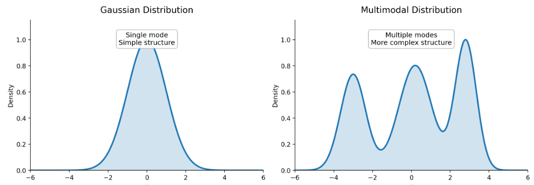
There are multiple, highly probable correct answers. In statistics, this means the data has multiple peaks (modes). Standard statistical models (like Gaussian distribution) are too simple for real-world data (one have one peak).
Hence, we need a way to represent complex, multimodal datasets.

8.2 Latent Variable Models

8.2.1 Definition and Efficient Representation

Because real-world data cannot be effectively modelled with simple probability distributions, we use latent variables. We assume that the observable data is generated by a smaller set of underlying, unobservable factors.
Notations:

1. Observation, $x$: The raw, complex data (like pixels of an image or words in a sentence).

2. Latent variable, $z$: hidden, unobserved factor that acts as an essential, compressed representation of the observation $x$.

3. Joint distribution, $p(x,z) = p(x|z)p(z)$.

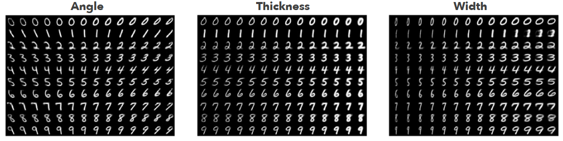
   • The prior $p(z)$: he distribution of the latent factors themselves. Before generating an image, the model randomly selects a set of traits from this distribution. For example, it might sample a $z$-vector that mathematically translates to "highly tilted" and "very thick".

   • Conditional distribution $p(x|z)$: Once the hidden traits ($z$) are chosen, this distribution determines the actual probability of the raw pixels ($x$) given those specific traits.

   • Data generation: To generate a new data point $x$, the model performs a two-step sampling process: first, sample $z \sim p(z)$, and then sample the image $x \sim p(x|z)$.

For example, each image (one digit) in the MNIST database is $28\times 28$ pixels. The raw observation $x$ exists in 784-dimensional space, which is computationally massive and inefficient.
Out of all combinations of 784 pixels, actual handwritten digits occupy a very small fraction. The latent variable $z$ captures just the necessary semantic features needed to draw the digit in a much lower dimension.
Some $z$ factors might be "which digit is it?"; "How slanted is it?"; "How thick is the stroke?".
Arithmetic operations in the latent space can admit meaningful semantic interpretations, in contrast to pixel space, where direct image addition lacks semantic meaning.

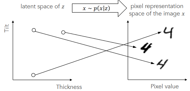
Here, $p(x|z)$ serves as the decoder of the encoder-decoder model. We feed a low-dimensional vector of numbers ($z$), and the network outputs a high-dimensional object ($x$). In contrast, the encoder would be represented by the posterior distribution $p(z|x)$.

8.2.2 The Manifold Hypothesis

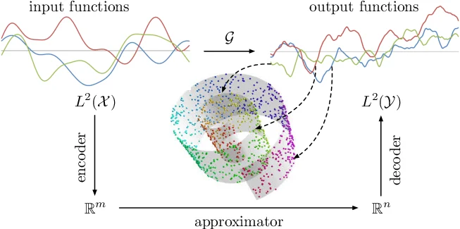
The Manifold Hypothesis says that high-dimensional, real-world data (like images or text) often lies on or near a lower-dimensional, structured manifold embedded within that high-dimensional space.
In the MNIST example, in the 84-dimensional space of a 28x28 pixel image, useful, structured data (like actual digits) tend to cluster along some lower-dimensional manifold within that space. Everywhere else in the higher-dimensional space, it is usually noise.
The implication is that we don’t need to waste computing power trying to learn the rules for the entire 784-dimensional space. Instead, we only need to learn the latent variable coordinates that map onto that manifold.

8.2.3 Gaussian Mixture Models (GMM)

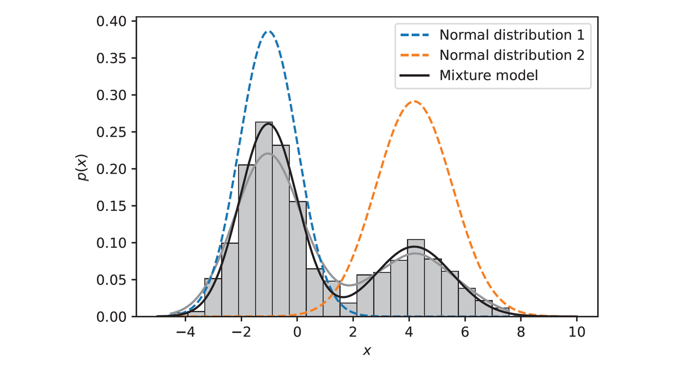
A Gaussian Mixture Model (GMM) is a probabilistic model assuming all data points are generated from a mixture of a finite number of Gaussian distributions with unknown parameters. It helps to solve our problem of modelling multiple peaks.
To create a GMM with $K$ different Gaussian distributions on a $d$-dimensional space ($\mathbb{R}^d$), the overall PDF is written as: $$p(x|\mu,\Sigma)=\sum_{t=1}^{K}\pi_{t}p(x|\mu_{t},\Sigma_{t})$$ ($d$ refers to the shape of the data, in the MNIST example, $d=784$)
The parameters:

• $\mu_{t} \in \mathbb{R}^d$: The mean (center) of the $t$-th Gaussian.

• $\Sigma_{t} \in \mathbb{R}^{d \times d}$: The covariance matrix (shape/spread) of the $t$-th Gaussian.

• $\pi_{t} \in [0,1]$: The mixing proportion (or weight) of the $t$-th Gaussian. This dictates how much "influence" that specific Gaussian has on the total mixture. The sum of all mixing proportions must equal 1 ($\sum_{t=1}^{K}\pi_{t}=1$).

The hyperparameter: The number of mixes, $K$. We have to decide how many clusters to look for before training the model.

The GMM is a specific type of latent variable model. We can translate the GMM equation into the $p(x, z)$ framework.
Here, the latent variable, $z$, answers the question: "Which specific Gaussian cluster did this data point come from?". Mathematically, $$z=(\zeta_{t})_{t=1}^{K} \in \{0,1\}^K,\quad \sum_{t=1}^{K}\zeta_{t}=1, \quad \zeta_t = \begin{cases} 1 & \text{if category } t \\ 0 & \text{otherwise} \end{cases}$$ This means $z$ is a one-hot vector of $K$ numbers where exactly one number is a ’1’ and the rest are ’0’s. For example, if we have $K=3$ clusters, and a data point was generated by the second Gaussian, then $z = (0, 1, 0)$.

We can represent the generation process $p(x, z) = p(x|z)p(z)$ using this $z$:

• The Prior $p(z)$: This is the probability of picking a specific cluster $t$ before we even look at the data. Note that this is just its mixing weight $\pi_t$. We write this as: $$p(z)=\prod_{t=1}^{K}\pi_{t}^{\zeta_{t}}$$ If $K=3$ and $z = [0, 1, 0]$, we get $(\pi_1^0) \times (\pi_2^1) \times (\pi_3^0) = 1 \times \pi_2 \times 1 = \pi_2$, which collapses down to just output the weight of the chosen cluster.

• The Conditional $p(x|z)$: This is the probability of generating data $x$, once we have chosen cluster $z$. We write this as: $$\prod_{t=1}^{K} p(x|\mu_t, \Sigma_t)^{\zeta_t}$$ Using the same example, we get $(Gaussian_1^0) \times (Gaussian_2^1) \times (Gaussian_3^0) = 1 \times Gaussian_2 \times 1$, which again isolates the PDF of the single chosen Gaussian.

• Marginal distribution of $x$: $$\begin{align*} p(x|\pi,\mu,\Sigma) &= \sum_z p(x,z|\pi,\mu,\Sigma) && \text{[Law of Total Probability]} \\ &= \sum_{t=1}^K p(x, \mathbf{1}_t|\pi,\mu,\Sigma) && \text{[$\mathbf{1}_t$ is a one-hot vector where the $t$-th slot is 1]} \\ &= \sum_{t=1}^K \pi_t p(x|\mu_t, \Sigma_t) && \text{[Using $p(x, z) = p(z)p(x|z)$]} \end{align*}$$ Note that summing out $z$ reconstructs the original GMM equation. Using $z$ does not change the shape of the model.

8.3 Expectation-Maximization (EM) Algorithm

We want to run MLE on the latent variable model to get the best values for the parameters $\mu$ (means), $\Sigma$ (covariances) and $\pi$ (mixing weights), so we have a decoder.

8.3.1 Intractability of Direct MLE

8.3.1.1 Why do we need to use the latent variable $z$?

Recall the MLE equation: $$\text{Total Log-Likelihood} = \sum_{i=1}^{n} \log p_{\theta}(X_i)$$ If we apply MLE on the GMM equation by only looking at $x$, we get $$\text{Total Log-Likelihood} = \sum_{i=1}^{n} \log \left( \sum_{t=1}^{K} \pi_t p(x|\mu_t, \Sigma_t) \right)$$ Taking the derivative is algebraically intractable. In other words, it is hard to simplify this as the summation is in the log.
What if know $z$ for every data point?
If we consider the joint probability $p(x, z)$, we have $$\begin{align*} \text{Total Log-Likelihood} &= \sum_{i=1}^n \log (p(x_i, z_i)) \\ &= \sum_{i=1}^n \log \left( \prod_{t=1}^K \left[ \pi_t \cdot p(x_i | \mu_t, \Sigma_t) \right]^{\zeta_{it}} \right) \end{align*}$$ This equation is easier to simplify as the product is in the log, so by properties of logarithms, the summation will be outside of the log.

8.3.2 The EM Framework (E-step and M-step)

However, to use $p(x, z)$ (to simplify the MLE equation above), we need to know the value of $\zeta_t$ (and by extension, $z$).
The EM algorithm is a way to find a MLE for problems where we have latent variables, i.e. $p(x|\theta) = \sum_z p(x,z|\theta)$.
The overarching flow is to iteratively improve our guess of the parameters $\theta$. We start with a completely random guess $\theta^{(1)}$, then use EM algorithm to find a better guess. $$\theta^{(1)} \rightarrow \theta^{(2)} \dots \rightarrow \theta^{(k)} \rightarrow \theta^{(k+1)} \dots$$ We have i.i.d. observations $x_{1:n} = (x_i)^n_{i=1}$, and note that $p(z_{1:n}|x_{1:n},\theta) = \prod_i p(z_i|x_i,\theta)$.
Recall that we wanted to maximise the true log-likelihood of our data: $$\log p(x_{1:n}|\theta) = \log \left( \sum_{z_{1:n}} p(x_{1:n}, z_{1:n}|\theta) \right)$$ But the problem is that there is a summation inside the log, making this algebraically intractable.

8.3.2.1 The E-step

We cannot directly optimize the likelihood because we do not know the hidden variables $z$. In this step, we use our current, locked-in parameter guesses $\theta^{(k)}$ to evaluate the probabilities of the hidden variables. Mathematically, this involves constructing a surrogate lower-bound function (which will become the Q-function) that approximates the true log-likelihood.
Jensen’s Inequality: For random variable $X$ and concave function $f$ ($\cap$ frown shape function), $$f(\mathbb{E}[X]) \ge \mathbb{E}[f(X)]$$ $$\begin{align*} \log p(x_{1:n}|\theta) &= \log \left( \sum_{z_{1:n}} p(z_{1:n}|x_{1:n}, \theta^{(k)}) \frac{p(x_{1:n}, z_{1:n}|\theta)}{p(z_{1:n}|x_{1:n}, \theta^{(k)})} \right) && \text{[Multiply and divide by posterior]} \\ &\ge \sum_{\textstyle z_{1:n}} p(z_{1:n}|x_{1:n}, \theta^{(k)}) \log \frac{p(x_{1:n}, z_{1:n}|\theta)}{p(z_{1:n}|x_{1:n}, \theta^{(k)})} && \text{[Jensen's inequality; $f$=$\log$, $\mathbb{E}$=$\textstyle\sum$]} \\ &= L(\theta, \theta^{(k)}) && \text{[Define a surrogate function]} \end{align*}$$ Note that we defined a surrogate function $L(\theta, \theta^{(k)})$. $$L(\theta, \theta^{(k)}) = \sum_{z_{1:n}} \underbrace{p(z_{1:n}|x_{1:n}, \theta^{(k)})}_{\text{Part 1}} \log \frac{\overbrace{p(x_{1:n}, z_{1:n}|\theta)}^{\text{Part 2}}}{\underbrace{p(z_{1:n}|x_{1:n}, \theta^{(k)})}_{\text{Part 3}}}$$

• Part 2 is the complete-data joint probability. This is the algebraically easier to solve equation, and we want to optimise this, but we need to know the hidden $z$.

• Part 1 acts as the weight, such that Part 1 $\times$ Part 2 gives expected value.

• Part 3 is the same term as Part 1, and acts as a normalisation constant to ensure the lower bound perfectly touches our current position.

2 properties of $L(\theta, \theta^{(k)})$:

1. $L(\theta, \theta^{(k)}) \le \log p(x_{1:n}|\theta)$. $L$ is guaranteed to be a lower bound that always sits underneath the true log-likelihood.

2. $L(\theta^{(k)},\theta^{(k)}) = \log p(x_{1:n|\theta^{(k)}})$. When $\theta = \theta^{(k)}$, $L$ perfectly equals the true log-likelihood.
   Derivation: $$\begin{align*} L(\theta^{(k)}, \theta^{(k)}) &= \sum_{z_{1:n}} p(z_{1:n}|x_{1:n}, \theta^{(k)}) \log \frac{p(x_{1:n}, z_{1:n}|\theta^{(k)})}{p(z_{1:n}|x_{1:n}, \theta^{(k)})} \\ &= \sum_{z_{1:n}} p(z_{1:n}|x_{1:n}, \theta^{(k)}) \log \frac{p(x_{1:n}|\theta^{(k)}) p(z_{1:n}|x_{1:n}, \theta^{(k)})}{p(z_{1:n}|x_{1:n}, \theta^{(k)})} && \text{[$p(x, z) = p(x)p(z|x)$]}\\ &= \sum_{z_{1:n}} p(z_{1:n}|x_{1:n}, \theta^{(k)}) \log p(x_{1:n}|\theta^{(k)}) \\ &= 1 \times \log p(x_{1:n}|\theta^{(k)}) &&\text{[$\log p(x_{1:n}|\theta^{(k)})$ is a constant]} \end{align*}$$

Getting the Q-function: $$\begin{align*} L(\theta^{(k)}, \theta^{(k)}) &= \sum_{\textstyle z_{1:n}} p(z_{1:n}|x_{1:n}, \theta^{(k)}) \log \frac{p(x_{1:n}, z_{1:n}|\theta)}{p(z_{1:n}|x_{1:n}, \theta^{(k)})} \\ &= \sum_z p(z_{1:n}|x_{1:n}, \theta^{(k)}) \Big[ \log p(x_{1:n}, z_{1:n}|\theta) - \log p(z_{1:n}|x_{1:n}, \theta^{(k)}) \Big] \\ &= \underbrace{\sum_z p(z|x, \theta^{(k)}) \log p(x, z|\theta)}_{\text{Term 1}} - \underbrace{\sum_z p(z_{1:n}|x_{1:n}, \theta^{(k)}) \log p(z_{1:n}|x_{1:n}, \theta^{(k)})}_{\text{Term 2}} \\ &= \sum_{z} p(z_{1:n}|x_{1:n}, \theta^{(k)}) \log p(x_{1:n}, z_{1:n}|\theta) \\ &= Q(\theta, \theta^{(k)}) \end{align*}$$

8.3.2.2 The M-step

Now we have a surrogate function built using our expectations of the hidden variables. The goal of the M-step is to find the brand new parameters ($\theta$) that maximize the Q function. We take the derivative of the Q-function with respect to our parameters $\theta$ and solve for zero to find the brand new, updated parameters $\theta^{(k+1)}$.

Note that Term 2 does not contain $\theta$, it only contains $\theta^{(k)}$ (our old, locked-in guesses), so we can discard it from the Q-function.
A more tractable form of the Q-function is: $$\begin{align*} Q(\theta, \theta^{(k)}) &= \sum_{z_{1:n}} p(z_{1:n}|x_{1:n}, \theta^{(k)}) \log \left( \prod_{i=1}^n p(x_i, z_i|\theta) \right) \\ &= \sum_{z_{1:n}} p(z_{1:n}|x_{1:n}, \theta^{(k)}) \sum_{i=1}^n \log p(x_i, z_i|\theta) \\ &= \sum_{i=1}^n \sum_{z_i} p(z_i|x_i, \theta^{(k)}) \log p(x_i, z_i|\theta) \end{align*}$$

• $\sum_{i=1}^n$ is a for loop over the dataset

• $\sum_{z_i}$ is a for loop over the clusters

• $p(z_i|x_i, \theta^{(k)})$ is the current guess for that single data point

• $\log p(x_i, z_i|\theta)$ is the complete-data log-likelihood for that single data point.

8.3.3 Application to Gaussian Mixtures

The Q-function is $$Q(\theta,\theta^{(k)})=\sum_{i=1}^{n}\sum_{z_{i}}p(z_{i}|x_{i},\theta^{(k)})\log p(x_{i},z_{i}|\theta)$$ For a GMM, the parameters $\theta$ consist of the mixing weights ($\pi$), the means ($\mu$), and the covariance matrices ($\Sigma$) for all $K$ clusters. Therefore, $\theta = (\pi, \mu, \Sigma)$ and for a specific cluster $t$, $\theta_t = (\pi_t, \mu_t, \Sigma_t)$.

8.3.3.1 The E-step

In this step, the goal is to use our current best guess of the parameters, denoted as $\theta^{(k)}$, to compute the probability that a specific data point $x_i$ came from a specific cluster $t$.
This probability is called the responsibility, denoted as $\gamma_{t,i}^{(k)}$. We calculate it using Bayes’ Theorem: $$\gamma_{t,i}^{(k)} = \frac{\pi_t^{(k)} p(x_i | \theta_t^{(k)})}{\sum_{s=1}^K \pi_s^{(k)} p(x_i | \theta_s^{(k)})}$$

• Numerator: The probability of picking cluster $t$ ($\pi_t$) multiplied by the Gaussian probability density of point $x_i$ under cluster $t$’s current mean and covariance.

• Denominator: The sum of that exact same calculation across all $K$ clusters. This normalizes the values so that the responsibilities for a single point $x_i$ add up to exactly 1.

8.3.3.2 The M-step

We plug these responsibilities into a surrogate function called the Q-function. The Q-function acts as a lower bound to our true, intractable log-likelihood. By maximizing the Q-function, we push the true likelihood up.
The Q-function for a GMM looks like this: $$Q(\theta, \theta^{(k)}) = \sum_{i=1}^n \sum_{t=1}^K \gamma_{t,i}^{(k)} \{\log \pi_t + \log p(x_i | \theta_t)\}$$ We now take the derivatives of the Q-function with respect to our parameters ($\pi_t, \mu_t, \Sigma_t$), set them to zero, and solve. This gives us the exact formulas to update our clusters to fit the data better, treating the responsibilities $\gamma_{t,i}^{(k)}$ as fixed weights.
First, we calculate the "effective number of points" assigned to cluster $t$ by summing up all the responsibilities for that cluster: $$n_t^{(k+1)} = \sum_{i=1}^n \gamma_{t,i}^{(k)}$$ Then, we use $n_t^{(k+1)}$ to calculate our brand new parameters, $\theta^{(k+1)}$:

1. Update the Mixing Weights: $$\pi_t^{(k+1)} = \frac{n_t^{(k+1)}}{n}$$ The new weight is simply the effective number of points in cluster $t$ divided by the total number of points $n$.

2. Update the Means: $$\mu_t^{(k+1)} = \frac{1}{n_t^{(k+1)}} \sum_{i=1}^n \gamma_{t,i}^{(k)} x_i$$ The new center is a weighted average of all data points. Points with a high responsibility $\gamma$ for this cluster pull the mean closer to themselves.

3. Update the Covariance Matrices: $$\Sigma_t^{(k+1)} = \frac{1}{n_t^{(k+1)}} \sum_{i=1}^n \gamma_{t,i}^{(k)} (x_i - \mu_t^{(k+1)})(x_i - \mu_t^{(k+1)})^\top$$ The new shape is a weighted covariance calculation. Notice the use of the outer product $(x_i - \mu)(x_i - \mu)^\top$ which gives us the required matrix structure, scaled by how much each point belongs to the cluster.

We now have a new set of parameters $\theta^{(k+1)}$. These are fed back into the E-step to calculate fresh responsibilities, which are then fed again into the M-step to get even better parameters.
This is repeated until the parameters stop changing significantly, at which point the algorithm has converged and the best fitting Gaussian distribution has been found.