5 Variance

For a random variable XX, the variance is Var(X)=๐•[X]=๐”ผ[(Xโˆ’๐”ผ[X])2]=๐”ผ[X2]โˆ’(๐”ผ[X])2\begin{align*} \text{Var}(X)=\mathbb{V}[X] &= \mathbb{E}[(X - \mathbb{E}[X])^2] \\ &=\mathbb{E}[X^2] - (\mathbb{E}[X])^2 \end{align*}

Variance measures the average of the squared distances from the mean.

Standard deviation is ฯƒ=๐•[X]\sigma = \sqrt{\mathbb{V}[X]}

For a constant cc,

  1. ๐•[c]=0\mathbb{V}[c]=0
    โˆต๐”ผ[(cโˆ’๐”ผ[c])2]=๐”ผ[(cโˆ’c)2]=๐”ผ[0]=0\because\mathbb{E}[(c-\mathbb{E}[c])^2]=\mathbb{E}[(c-c)^2]=\mathbb{E}[0]=0

  2. ๐•[X+c]=๐•[X]\mathbb{V}[X+c] = \mathbb{V}[X]
    โˆต๐”ผ[((X+c)โˆ’๐”ผ[X+c])2]=๐”ผ[(X+cโˆ’(๐”ผ[X]+c))2]=๐”ผ[(Xโˆ’๐”ผ[X])2]\because\mathbb{E}[((X+c)-\mathbb{E}[X+c])^2]=\mathbb{E}[(X+c-(\mathbb{E}[X]+c))^2]=\mathbb{E}[(X-\mathbb{E}[X])^2]

  3. ๐•[cX]=c2๐•[X]\mathbb{V}[cX]=c^2\mathbb{V}[X]
    โˆต๐”ผ[(cXโˆ’๐”ผ[cX])2]=๐”ผ[(cXโˆ’c๐”ผ[X])2]=๐”ผ[c2(Xโˆ’๐”ผ[X])2]=c2๐”ผ[(Xโˆ’๐”ผ[X])2]\because\mathbb{E}[(cX-\mathbb{E}[cX])^2]=\mathbb{E}[(cX-c\mathbb{E}[X])^2]=\mathbb{E}[c^2(X-\mathbb{E}[X])^2]=c^2\mathbb{E}[(X-\mathbb{E}[X])^2]

5.1 Covariance

For random variables XX, YY, Cov(X,Y)=๐”ผ[(Xโˆ’๐”ผ[X])(Yโˆ’๐”ผ[Y])]=๐”ผ[XY]โˆ’๐”ผ[X]๐”ผ[Y]\begin{align*} \text{Cov}(X,Y)&=\mathbb{E}[(X-\mathbb{E}[X])(Y-\mathbb{E}[Y])] \\ &= \mathbb{E}[XY]-\mathbb{E}[X]\mathbb{E}[Y] \end{align*}

Note that Variance is a specific case of Covariance, i.e. Cov(X,X)=๐•[X]\text{Cov}(X,X)=\mathbb{V}[X]

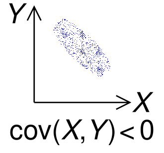
XX and YY move inversely.
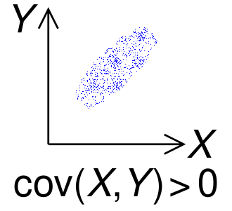
XX and YY move together.
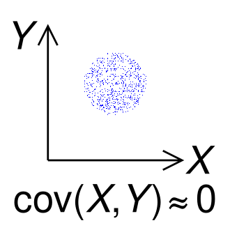
No linear pattern.

For random variables XX, YY and constants c1c_1, c2c_2, ๐•[c1X+c2Y]=c12๐•[X]+c22๐•[Y]+2c1c2๐”ผ[(Xโˆ’๐”ผ[X])(Yโˆ’๐”ผ[Y])]=c12๐•[X]+c22๐•[Y]+2c1c2Cov(X,Y)\begin{align*} \mathbb{V}[c_1X+c_2Y]&=c_1^2\mathbb{V}[X]+c_2^2\mathbb{V}[Y]+2c_1c_2\mathbb{E}[(X-\mathbb{E}[X])(Y-\mathbb{E}[Y])] \\ &=c_1^2\mathbb{V}[X]+c_2^2\mathbb{V}[Y]+2c_1c_2\text{Cov}(X,Y) \end{align*}

Proof.
๐•[c1X+c2Y]=๐”ผ[((c1X+c2Y)โˆ’(c1๐”ผ[X]+c2๐”ผ[Y]))2]=๐”ผ[(c1(Xโˆ’๐”ผ[X])+c2(Yโˆ’๐”ผ[Y]))2]=๐”ผ[c12(Xโˆ’๐”ผ[X])2]+๐”ผ[c22(Yโˆ’๐”ผ[Y])2]+2c1c2(Xโˆ’๐”ผ[X])(Yโˆ’๐”ผ[Y])=c12๐•[X]+c22๐•[Y]+2c1c2Cov(X,Y)\begin{align*} \mathbb{V}[c_1X+c_2Y]&=\mathbb{E}[((c_1X+c_2Y)-(c_1\mathbb{E}[X]+c_2\mathbb{E}[Y]))^2] \\ &=\mathbb{E}[(c_1(X-\mathbb{E}[X])+c_2(Y-\mathbb{E}[Y]))^2] \\ &=\mathbb{E}[c_1^2(X-\mathbb{E}[X])^2]+\mathbb{E}[c_2^2(Y-\mathbb{E}[Y])^2]+2c_1c_2(X-\mathbb{E}[X])(Y-\mathbb{E}[Y]) \\ &=c_1^2\mathbb{V}[X] + c_2^2\mathbb{V}[Y] + 2c_1c_2\text{Cov}(X,Y) \end{align*}

The implication is that when Cov(X,Y)>0(X,Y)>0, ๐•(X+Y)>๐•(X)+๐•(Y)\mathbb{V}(X+Y)>\mathbb{V}(X)+\mathbb{V}(Y).

For example, if portfolio has multiple stocks that tend to move together (Cov), the combined portfolio is riskier. Conversely, the risk decreases if negatively correlated stocks are held together.

5.1.1 Independence

By extension, if XX and YY are independent, Cov(X,Y)=0(X,Y)=0. Then, ๐•[X+Y]=๐•[X]+๐•[Y]\mathbb{V}[X+Y]=\mathbb{V}[X]+\mathbb{V}[Y]

However, zero Covariance does not imply independence.
For example, let random variable XX take three values:

  1. P(X=โˆ’1)=13P(X=-1)=\frac{1}{3}

  2. P(X=0)=13P(X=0)=\frac{1}{3}

  3. P(X=1)=13P(X=1)=\frac{1}{3}

Let Y=X2Y=X^2.
We know that YY is dependent on XX.
Calculating covariance,
We have ๐”ผ[X]=โˆ’1+0+13=0\mathbb{E}[X]=\frac{-1+0+1}{3}=0.
Calculating XYXY,

So ๐”ผ[XY]=โˆ’1+0+13=0\mathbb{E}[XY]=\frac{-1+0+1}{3}=0
Therefore, Cov(X,Y)=๐”ผ[XY]โˆ’๐”ผ[X]๐”ผ[Y]=0\begin{align*} \text{Cov}(X,Y)&=\mathbb{E}[XY]-\mathbb{E}[X]\mathbb{E}[Y] \\ &=0 \end{align*}

Takeaway: Covariance only tests for linear relationships. For non-linear cases like Y=X2Y=X^2, Covariance might be 0 even though the variables are dependent on each other.

5.2 Variance-covariance matrix

[๐•[X]Cov(X,Y)Cov(X,Z)Cov(Y,X)๐•[Y]Cov(Y,Z)Cov(Z,X)Cov(Z,Y)๐•[Z]]\begin{bmatrix} \mathbb{V}[X] & \text{Cov}(X, Y) & \text{Cov}(X, Z) \\ \text{Cov}(Y, X) & \mathbb{V}[Y] & \text{Cov}(Y, Z) \\ \text{Cov}(Z, X) & \text{Cov}(Z, Y) & \mathbb{V}[Z] \end{bmatrix}

5.3 Correlation coefficient

ฯX,Y=Cov(X,Y)ฯƒXฯƒY\rho_{X,Y} = \frac{\text{Cov}(X, Y)}{\sigma_X \sigma_Y} where ฯƒX\sigma_X and ฯƒY\sigma_Y, the standard deviations of XX and YY, are the normalisation factor.

Thus, we have ฯX,Yโˆˆ[โˆ’1,1]\rho_{X,Y}\in[-1,1], by Cauchy-Schwarz inequality.

For example, two random variables YY and XX have the strongest linear relationship when Y=XY=X. Then Cov(X,Y)=Cov(X,X)=ฯƒX2\text{Cov}(X,Y)=\text{Cov}(X,X)=\sigma_X^2 The correlation coefficient is ฯX,Y=ฯƒX2ฯƒX2=1\rho_{X,Y}=\frac{\sigma_X^2}{\sigma_X^2}=1

5.4 Change of Variables

5.4.1 PMF (Discrete case)

Let XX be a random variable with PMF pX(x)p_X(x).
Let Y=g(X)Y=g(X).
Then the PMF of YY is obtained by summing up all the original xx values that transform into that yy. pY(y)=โˆ‘x:g(x)=ypX(x)p_Y(y)=\sum_{x:g(x)=y}p_X(x) Examples:

5.4.2 PDFs (Continuous case, single variable)

Define random variables XX and Y=g(X)Y=g(X), where gg is continuously differentiable and one-to-one.
Then the PDFs fXf_X and fYf_Y satisfy fX(x)=fY(g(x))|dg(x)dx|f_X(x)=f_Y(g(x))\left|\frac{\mathrm{d}g(x)}{\mathrm{d}x}\right| |dg(x)dx|\left|\frac{\mathrm{d}g(x)}{\mathrm{d}x}\right| here is the scaling factor.

Proof. By definition, the Cumulative Distribution Function (CDF) is FX(x)=P(Xโ‰คx)F_X(x) = P(X \leq x)

Case 1: g(x)g(x) is strictly increasing.
The inequality is preserved: P(Xโ‰คx)=P(g(X)โ‰คg(x))=P(Yโ‰คg(x))=FY(g(x))P(X \leq x) = P(g(X) \leq g(x)) = P(Y \leq g(x)) = F_Y(g(x)) So, we have the identity FX(x)=FY(g(x))F_X(x) = F_Y(g(x))

To obtain the PDF, we differentiate both sides with respect to xx.
On the right side, we apply the Chain Rule: ddxFX(x)=ddxFY(g(x))\frac{d}{dx} F_X(x) = \frac{d}{dx} F_Y(g(x)) fX(x)=fY(g(x))โ‹…gโ€ฒ(x)f_X(x) = f_Y(g(x)) \cdot g'(x) Since gg is increasing, gโ€ฒ(x)>0g'(x) > 0, so this matches our formula.

Case 2: If g(x)g(x) were strictly decreasing, the inequality would flip (Xโ‰คxโ‡”Yโ‰ฅg(x)X \leq x \iff Y \geq g(x)), leading to a negative sign.
To cover both cases, we take the absolute value of the derivative:

fX(x)=fY(g(x))โ‹…|dg(x)dx|f_X(x) = f_Y(g(x)) \cdot \left| \frac{dg(x)}{dx} \right|

Intuitive explanation.
In a PDF, since probability is area, the probability mass in a tiny interval of XX must equal the probability mass in the corresponding interval of YY. fX(x)โ‹…dx=fY(y)โ‹…dyf_X(x) \cdot dx = f_Y(y) \cdot dy

The relationship between the interval widths (dydy vs dxdx) is determined by the derivative (the slope of the transformation): dydx=gโ€ฒ(x)โŸนdy=gโ€ฒ(x)โ‹…dx\frac{dy}{dx} = g'(x) \implies dy = g'(x) \cdot dx

Substitute dydy back into the area equation: fX(x)โ‹…dx=fY(y)โ‹…(gโ€ฒ(x)โ‹…dxโŸdy)fX(x)=fY(y)โ‹…gโ€ฒ(x)\begin{align*} f_X(x) \cdot dx &= f_Y(y) \cdot (\underbrace{g'(x) \cdot dx}_{dy}) \\ f_X(x) &= f_Y(y) \cdot g'(x) \end{align*} To ensure the density is positive (even if g(x)g(x) is decreasing), we take the absolute value of the derivative: fX(x)=fY(g(x))โ‹…|dg(x)dx|f_X(x) = f_Y(g(x)) \cdot \left| \frac{dg(x)}{dx} \right|

Example. Y=aX+bโ†’fX(x)=|a|fY(ax+b)Y=aX+b\rightarrow f_X(x)=|a|f_Y(ax+b).

5.4.3 PDFs (Continuous case, multiple variables)

Let X1,โ€ฆ,XnX_1,\ldots,X_n be nn continuous random variables, transformed to nn new random variables Y1,โ€ฆ,YnY_1,\ldots, Y_n using a set of functions Yi=gi(X1,X2,โ€ฆ,Xn),for iโˆˆ[1,โ€ฆ,n]Y_i=g_i(X_1,X_2,\ldots,X_n)\:, \quad \text{for } i \in [1,\ldots,n] We then have a Jacobian matrix of size nร—nn\times n. J=(โˆ‚y1โˆ‚x1โ‹ฏโˆ‚y1โˆ‚xnโ‹ฎโ‹ฑโ‹ฎโˆ‚ynโˆ‚x1โ‹ฏโˆ‚ynโˆ‚xn)J = \begin{pmatrix} \frac{\partial y_1}{\partial x_1} & \cdots & \frac{\partial y_1}{\partial x_n} \\ \vdots & \ddots & \vdots \\ \frac{\partial y_n}{\partial x_1} & \cdots & \frac{\partial y_n}{\partial x_n} \end{pmatrix} Each row ii tells us how each output YiY_i changes as any of the inputs X1,โ€ฆ,XnX_1,\ldots,X_n change. While in single variable calculus, the derivative is just a single number (the slope), for multivariable calculus, the Jacobian matrix is the collection of all the slopes at once.
Then, the Jacobian determinant replaces gโ€ฒ(x)g'(x) in the 1D case. It tells us how much the volume is transformed.

The joint PDFs fX1,โ€ฆ,Xnf_{X_1,\ldots,X_n} and fY1,โ€ฆ,Ynf_{Y1,\ldots,Y_n} satisfy fX1,โ€ฆ,Xn(x1,โ€ฆ,xn)=fY1,โ€ฆ,Yn(g1(x),โ€ฆ,gn(x))โ‹…|det⁡J(x1,โ€ฆ,xn)|f_{X_1,\ldots,X_n}(x_1,\ldots,x_n)=f_{Y1,\ldots,Y_n}(g_1(x),\ldots,g_n(x))\cdot |\det J(x_1,\ldots,x_n)| where |det⁡J(x1,โ€ฆ,xn)||\det J(x_1,\ldots,x_n)| represents the absolute value of the determinant of the nร—nn\times n Jacobian matrix. This number represents the volume scaling factor of the transformation in nn-dimensional space.

In vector notation, with ๐‘ฟ=(X1,โ€ฆ,Xn)\mathbf{X}=(X_1,\ldots,X_n), ๐’€=(Y1,โ€ฆ,Yn)\mathbf{Y}=(Y_1,\ldots,Y_n), ฯ†=(g1,โ€ฆ,gn)\varphi=(g_1,\ldots,g_n), fX(x)=fY(ฯ†(x))|det⁡Jฯ†(x)|f_X(x)=f_Y(\varphi(x))|\det J_{\varphi}(x)| In terms of fYf_Y, fY(y)=fX(inverse of x)โ‹…1|det⁡A|f_Y(y)=f_X(\text{inverse of x})\cdot \frac{1}{|\det A|}

Example. Y=AX+bโ†’fX(x)=fY(AX+b)|det⁡A|Y=AX+b \rightarrow f_X(x)=f_Y(AX+b)|\det A|.

5.4.4 Gaussian distribution - Change of variable

Let XX follow the Gaussian distribution N(ฮผ,ฯƒ2)N(\mu, \sigma^2), fX(x)=12ฯ€ฯƒ2eโˆ’(xโˆ’ฮผ)22ฯƒ2.f_X(x) = \frac{1}{\sqrt{2\pi\sigma^2}} e^{-\frac{(x-\mu)^2}{2\sigma^2}}.

Change of variable: Y=aX+bY = aX + b. Then, fX(x)=|a|fY(ax+b)โ‡”fY(y)=1|a|fX(yโˆ’ba)โ‡”fY(y)=12ฯ€a2ฯƒ2exp⁡(โˆ’(yโˆ’(aฮผ+b))22a2ฯƒ2)โ‡”fY(y)=N(aฮผ+b,a2ฯƒ2)\begin{align*} & f_X(x) = |a| f_Y(ax + b) \\ \iff & f_Y(y) = \frac{1}{|a|} f_X \left( \frac{y - b}{a} \right) \\ \iff & f_Y(y) = \frac{1}{\sqrt{2\pi a^2 \sigma^2}} \exp(-\frac{(y - (a\mu + b))^2}{2a^2 \sigma^2}) \\ \iff & f_Y(y) = N(a\mu + b, a^2 \sigma^2) \end{align*}

Takeaway: If we apply a linear transformation to a Gaussian random variable, the result is also a Gaussian distribution.

5.4.5 Multivariate Gaussian distribution - Change of variable

Let X1X_1 and X2X_2 independently follow the standard Gaussian distribution N(0,1)N(0,1). fX1(x1)=12ฯ€exp⁡(โˆ’x22)f_{X_1}(x_1)=\frac{1}{\sqrt{2\pi}}\exp(\frac{-x^2}{2}) The joint PDF of (X1,X2X_1,X_2) is fX1,X2(x1,x2)=(12ฯ€exp⁡(โˆ’x22))(12ฯ€exp⁡(โˆ’x22))=12ฯ€exp⁡(โˆ’x12+x222)f_{X_1,X_2}(x_1,x_2)=(\frac{1}{\sqrt{2\pi}}\exp(\frac{-x^2}{2}))(\frac{1}{\sqrt{2\pi}}\exp(\frac{-x^2}{2}))=\frac{1}{2\pi}\exp(-\frac{x_1^2+x_2^2}{2}) Generalising to dd-variate standard Gaussian distribution N(๐ŸŽ,Id)N(\mathbf{0},I_d), fX(x)=1(2ฯ€)d/2exp⁡(โˆ’xdTxd2)f_X(x)=\frac{1}{(2\pi)^{d/2}}\exp(-\frac{x_d^Tx_d}{2}) Here, xdTxd=[x1x2โ‹ฏxd]โ‹…[x1x2โ‹ฎxd]=x12+x22+โ‹ฏ+xd2x_d^Tx_d = \begin{bmatrix} x_1 & x_2 & \cdots & x_d \end{bmatrix} \cdot \begin{bmatrix} x_1 \\ x_2 \\ \vdots \\ x_d \end{bmatrix} = x_1^2 + x_2^2 + \cdots + x_d^2.
Also, the covariance matrix Id=[10โ‹ฏ001โ‹ฏ0โ‹ฎโ‹ฎโ‹ฑโ‹ฎ00โ‹ฏ1]I_d = \begin{bmatrix} 1 & 0 & \cdots & 0 \\ 0 & 1 & \cdots & 0 \\ \vdots & \vdots & \ddots & \vdots \\ 0 & 0 & \cdots & 1 \end{bmatrix}, meaning the variance of each variable is 1, and there is zero covariance between any of the variables.

Letting XX follow N(๐ŸŽ,Id)N(\mathbf{0},I_d), we apply a change of variables Y=AX+ฮผY=AX+\mu, where ฮผโˆˆโ„d\mu\in\mathbb{R}^d.
ฮผ\mu is basically a vector of dd numbers.
To find the PDF of YY, apply the change of variables formula: fY(y)=fX(inverse x)โ‹…1|det⁡A|f_Y(y)=f_X(\text{inverse }x)\cdot \frac{1}{|\det A|} Since X=Aโˆ’1(Yโˆ’ฮผ),X=A^{-1}(Y-\mu), Substituting in, we get fY(y)=1|det⁡A|โ‹…1(2ฯ€)d/2exp⁡(โˆ’12[Aโˆ’1(yโˆ’ฮผ)]T[Aโˆ’1(yโˆ’ฮผ)])f_Y(y)=\frac{1}{|\det A|}\cdot \frac{1}{(2\pi)^{d/2}}\exp(-\frac{1}{2}[A^{-1}(y-\mu)]^T[A^{-1}(y-\mu)]) Defining the new covariance matrix as ฮฃ=AAT\Sigma = AA^T, we have det⁡(ฮฃ)=det⁡(A)det⁡(AT)=(det⁡(A))2โ‡’|det⁡A|=det⁡ฮฃ\det(\Sigma)=\det(A)\det(A^T)=(\det(A))^2\Rightarrow |\det A|=\sqrt{\det\Sigma} and [Aโˆ’1(yโˆ’ฮผ)]T=(yโˆ’ฮผ)T(Aโˆ’1)Tโ‡’[Aโˆ’1(yโˆ’ฮผ)]T[Aโˆ’1(yโˆ’ฮผ)]=(yโˆ’ฮผ)T(Aโˆ’1)TAโˆ’1(yโˆ’ฮผ)=(yโˆ’ฮผ)Tฮฃโˆ’1(yโˆ’ฮผ)\begin{align*} [A^{-1}(y-\mu)]^T &= (y-\mu)^T(A^{-1})^T \\ \Rightarrow [A^{-1}(y-\mu)]^T[A^{-1}(y-\mu)] &= (y-\mu)^T(A^{-1})^TA^{-1}(y-\mu) \\ &= (y-\mu)^T\Sigma^{-1}(y-\mu) \end{align*}

Finally, we get fY(y)=1(2ฯ€)d/2|det⁡ฮฃ|exp⁡(โˆ’12(yโˆ’ฮผ)โŠคฮฃโˆ’1(yโˆ’ฮผ))f_Y(y) = \frac{1}{(2\pi)^{d/2} \sqrt{|\det \Sigma|}} \exp\left( -\frac{1}{2} (y - \mu)^\top \Sigma^{-1} (y - \mu) \right) Comparing to the d-variate standard Gaussian distribution N(๐ŸŽ,Id)N(\mathbf{0},I_d),
the d-variate Gaussian distribution fX(x)f_X(x) is N(ฮผ,ฮฃ)N(\mu, \Sigma), where ๐”ผ[X]=ฮผ\mathbb{E}[X]=\mu and ฮฃ=AAT\Sigma=AA^T is the variance-covariance matrix.

5.5 Moments

For a random variable XX, the kk-th momemnt is ฮผk=๐”ผ[Xk]\mu_k=\mathbb{E}[X^k] Each subsequent moment provides more information about the structure of the distribution.
For example,
The first moment tells us about the mean, the second moment tells us about the variance, ๐”ผ[X]=ฮผ1๐•[X]=๐”ผ[X2]โˆ’(๐”ผ[X])2=ฮผ2โˆ’ฮผ12\mathbb{E}[X] = \mu_1\quad\mathbb{V}[X] = \mathbb{E}[X^2]-(\mathbb{E}[X])^2=\mu_2-\mu_1^2 The third moment tells us about skewness, the fourth tells us about kurtosis, and so on.

A probability distribution is uniquely specified by its moment generating function (MGF). Note: It is not uniquely specified by its moments.

The moment generating function (MGF) is MX(t)=๐”ผ[etX]={โˆ‘xetxpX(x)(discrete),โˆซetxfX(x)dx(continuous).M_X(t) = \mathbb{E}[e^{tX}] = \begin{cases} \displaystyle \sum_{x} e^{tx} p_X(x) & (\text{discrete}), \\[15pt] \displaystyle \int e^{tx} f_X(x) \mathrm{d}x & (\text{continuous}). \end{cases}

We use ๐”ผ[etX]\mathbb{E}[e^{tX}] because from the taylor expansion of ee, etX=1+tX+(tX)22!+(tX)33!โ‹ฏe^{tX}=1+tX+\frac{(tX)^2}{2!}+\frac{(tX)^3}{3!}\cdots Taking expectation, MX(t)=๐”ผ[etX]=๐”ผ[1]+๐”ผ[tX]+๐”ผ[t2X22!]+โ‹ฏ=1+t๐”ผ[X]+t22!๐”ผ[X2]+t33!๐”ผ[X3]+โ‹ฏ\begin{align*} M_X(t)&=\mathbb{E}[e^{tX}]=\mathbb{E}[1]+\mathbb{E}[tX]+\mathbb{E}[\frac{t^2X^2}{2!}]+\cdots \\ &= 1 + t\mathbb{E}[X] + \frac{t^2}{2!}\mathbb{E}[X^2] + \frac{t^3}{3!}\mathbb{E}[X^3]+\cdots \end{align*} Therefore, by taking the kk-th derivative, MX(k)(t)=ฮผk+ฮผk+1t+ฮผk+22!t2+ฮผk+33!t3+โ‹ฏM_X^{(k)}(t)=\mu_k + \mu_{k+1}t + \frac{\mu_{k+2}}{2!}t^2 + \frac{\mu_{k+3}}{3!}t^3+\cdots and setting t=0t=0, we get the moments ฮผk=MX(k)(0)\mu_k=M_X^{(k)}(0)

5.5.1 Example for Gaussian distribution

For a Standard Normal Distribution (Zโˆผ๐’ฉ(0,1)Z \sim \mathcal{N}(0, 1)), the MGF is defined as MZ(t)=๐”ผ[etZ]=โˆซโˆ’โˆžโˆžetz12ฯ€eโˆ’z22dz=12ฯ€โˆซโˆ’โˆžโˆžeโˆ’12(z2โˆ’2tz)dz\begin{align*} M_Z(t) = \mathbb{E}[e^{tZ}] &= \int_{-\infty}^{\infty} e^{tz} \frac{1}{\sqrt{2\pi}} e^{-\frac{z^2}{2}} \, dz \\ &= \frac{1}{\sqrt{2\pi}} \int_{-\infty}^{\infty} e^{-\frac{1}{2}(z^2 - 2tz)} \, dz \end{align*}

We complete the square in the exponent: โˆ’12(z2โˆ’2tz)=โˆ’12(z2โˆ’2tz+t2โˆ’t2)=โˆ’12(zโˆ’t)2+t22-\frac{1}{2}(z^2 - 2tz) = -\frac{1}{2}(z^2 - 2tz + t^2 - t^2) = -\frac{1}{2}(z-t)^2 + \frac{t^2}{2}. Substituting this back into the integral: MZ(t)=12ฯ€โˆซโˆ’โˆžโˆžeโˆ’12(zโˆ’t)2+t22dz=et22โˆซโˆ’โˆžโˆž12ฯ€eโˆ’12(zโˆ’t)2dzโŸ=1\begin{align*} M_Z(t) &= \frac{1}{\sqrt{2\pi}} \int_{-\infty}^{\infty} e^{-\frac{1}{2}(z-t)^2 + \frac{t^2}{2}} \, dz \\ &= e^{\frac{t^2}{2}} \underbrace{\int_{-\infty}^{\infty} \frac{1}{\sqrt{2\pi}} e^{-\frac{1}{2}(z-t)^2} \, dz}_{=1} \end{align*} The integral is equal to 1 because it represents the total probability of a Normal distribution with mean tt and variance 11. Thus: MZ(t)=et2/2M_Z(t) = e^{t^2/2}

Then for a General Normal Distribution (Xโˆผ๐’ฉ(ฮผ,ฯƒ2)X \sim \mathcal{N}(\mu, \sigma^2)),

We use the linear transformation property X=ฮผ+ฯƒZX = \mu + \sigma Z: MX(t)=๐”ผ[etX]=๐”ผ[et(ฮผ+ฯƒZ)]=etฮผโ‹…๐”ผ[e(tฯƒ)Z](Since etฮผ is constant)=etฮผโ‹…MZ(tฯƒ)\begin{align*} M_X(t) &= \mathbb{E}[e^{tX}] \\ &= \mathbb{E}[e^{t(\mu + \sigma Z)}] \\ &= e^{t\mu} \cdot \mathbb{E}[e^{(t\sigma)Z}] \quad (\text{Since } e^{t\mu} \text{ is constant}) \\ &= e^{t\mu} \cdot M_Z(t\sigma) \end{align*}

Using the result MZ(u)=eu2/2M_Z(u) = e^{u^2/2} from Part 1 with u=tฯƒu = t\sigma: MX(t)=etฮผโ‹…e(tฯƒ)2/2=exp⁡(ฮผt+12ฯƒ2t2)\begin{align*} M_X(t) &= e^{t\mu} \cdot e^{(t\sigma)^2 / 2} \\ &= \exp\left(\mu t + \frac{1}{2}\sigma^2 t^2\right) \end{align*} The Gaussian distribution is characterised by only the mean and variance.

5.6 Poisson distribution

The Poisson distribution models the number of events occuring in some fixed interval (of time or space), given a constant average rate ฮป\lambda, independence of events.

For a random variable XX that follow a Poisson distribution, we write XโˆผPo(ฮป)X\sim \text{Po}(\lambda)

The Poisson distribution is basically a limit of the Binomial distribution B(n,p)B(n,p).
Recall that for XโˆผB(n,p)X\sim B(n,p), P(X=k)=(nk)pk(1โˆ’p)nโˆ’kP(X=k)=\binom{n}{k}p^k(1-p)^{n-k} Consider some time interval [0,t0,t] divided into nn tiny parts. Some event occurs on average ฮป\lambda times in [0,t0,t].
The probability of the event occuring in each of the nn parts is roughly ฮปn\frac{\lambda}{n}.
If nn is sufficiently large, each part can have at most one event.
Taking limit of the Binomial distribution as nโ†’โˆžn\rightarrow\infty, limnโ†’โˆž[(nk)โ‹…(ฮปn)kโ‹…(1โˆ’ฮปn)nโˆ’k]\lim\limits_{n\to \infty}\left[\binom{n}{k} \cdot (\frac{\lambda}{n})^k \cdot (1-\frac{\lambda}{n})^{n-k} \right] We get P(X=k)=eโˆ’ฮปโ‹…ฮปkk!P(X=k)=\frac{e^{-\lambda} \cdot \lambda^k}{k!} This is the probability that some event occurs kk times in [0,t0,t], given that it occurs ฮป\lambda times on average in [0,t0,t].

The MGF for some Poisson distribution is MX(t)=๐”ผ[etX]=โˆ‘k=0+โˆžetkโ‹…eโˆ’ฮปโ‹…ฮปkk!=eโˆ’ฮปโˆ‘k=0+โˆžetkฮปkk!=eโˆ’ฮปโˆ‘k=0+โˆž(etฮป)kk!=eโˆ’ฮปโ‹…eetโ‹…ฮป=eฮป(etโˆ’1)\begin{align*} M_X(t)=\mathbb{E}[e^{tX}]&=\sum_{k=0}^{+\infty}e^{tk}\cdot\frac{e^{-\lambda} \cdot \lambda^k}{k!}\\ &=e^{-\lambda}\sum_{k=0}^{+\infty}\frac{e^{tk}\lambda^k}{k!} \\ &=e^{-\lambda}\sum_{k=0}^{+\infty}\frac{(e^t\lambda)^k}{k!} \\ &=e^{-\lambda}\cdot e^{e^{t}\cdot \lambda} \\ &=e^{\lambda(e^t-1)} \end{align*}

Taking first and second derivatives of MX(t)M_X(t) and setting t=0t=0, ฮผ1=MXโ€ฒ(0)=ฮป,ฮผ2=MXโ€ณ(0)=ฮป+ฮป2\mu_1=M'_X(0)=\lambda, \quad \mu_2=M''_X(0)=\lambda + \lambda^2 Then ๐”ผ[X]=ฮผ1=ฮป,๐•[X]=ฮผ2โˆ’ฮผ12=ฮป\mathbb{E}[X]=\mu_1=\lambda, \quad \mathbb{V}[X]=\mu_2-\mu_1^2=\lambda Poisson distributionโ€™s mean and variance are both ฮป\lambda.