7 Estimation

Given indepedent observations $X_1, \ldots, X_n$ that come from some unknown, true probability distribution $P$, how do we infer $P$?

1. Moment Estimation: Estimate the mean and variance of the data.

2. Finding the full mathematical curve (the distribution) that best fits your dataset, bu tuning parameters. By learning this underlying shape, AI models can sample from it to generate new, realistic synthetic data.

3. Regression/Classification: Supervised learning, where the observations come in pairs. An input and its corresponding label, denoted as $(X_{i}, Y_{i})$. The goal is to estimate the relationship between them, such as predicting the conditional probability of a label given an input ($P_{Y|X}$) or the expected value ($\mathbb{E}[Y|X]$).

7.1 Estimator/Estimate

The primary goal of statistical inference (or learning) is to construct an estimator for $\theta_{*}$.
This $\theta_{*}$ represents a true, unknown parameter associated with a probability distribution $P$.
Examples of this parameter include the mean, the variance, or the parameter of a probabilistic model, $p_{\theta}$.
Estimator vs Estimate:

• Estimator: This is defined as a random variable, $\hat{\theta}$, that depends on your data observations ($X_{1},...X_{n}$). It is the overarching mathematical formula or rule, written as $\hat{\theta}=\hat{\theta}(X_{1},...X_{n})$.

• Estimate: This is the actual output you get when you plug specific, concrete data points ($x_{1},...,x_{n}$) into your estimator formula. It is the final calculated result, written as $\hat{\theta}(x_{1},...,x_{n})$.

The 4 criteria to evaluate if an estimator is good:

• Unbiasedness: An estimator $\hat{\theta}(X_{1},...X_{n})$ is unbiased for a true parameter $\theta$ if $\mathbb{E}[\hat{\theta}]=\theta$. The average of many estimates is the true answer.

• Consistency: An estimator $\hat{\theta}(X_{1},...X_{n})$ is consistent for a true parameter $\theta$ if $\forall \epsilon > 0,\:\lim\limits_{n\rightarrow\infty}P(|\hat{\theta}-\theta|\le\epsilon)=1$. A single estimate becomes perfectly accurate with enough data.

• Effectivity: An unbiased estimator is considered more effective if it has a lower variance than another unbiased estimator, i.e. the confidence is greater.

• Asymptotic normality: As $n \to \infty$, distribution of your estimator’s guesses will start to perfectly resemble a Normal Distribution (a classic bell curve) centered around the true parameter, by the CLT.

7.1.1 Bias-variance decomposition

When we create an estimator ($\hat{\theta}$) to guess a true, unknown parameter ($\theta_*$), we need a way to mathematically measure how "good" that guess is.
The motivation: Suppose you have independent data points $X_1, X_2, ..., X_n$ and you want to estimate the true mean.

1. $\hat{\theta}_1 = \frac{1}{n} \sum_{i=1}^n X_i$ (The sample mean, averaging $n$ data points).

2. $\hat{\theta}_2 = X_1$ (Just the first data point).

Both estimators are unbiased, i.e. if you repeat the experiment infinitely many times, both will eventually average out to the true mean.
However, intuitively, $\hat{\theta}_1$ is a much better estimator, as it uses all the data, meaning it will fluctuate much less from sample to sample. $\hat{\theta}_2$ will wildly jump around depending on what that first data point happens to be. ($\mathbb{V}[hat{\theta}_1] = \frac{\mathbb{V}[hat{\theta}_2]}{n}$).

The standard way to measure the quality of estimators by calculating the Expected Squared Error: $\mathbb{E}[||\hat{\theta} - \theta_*||^2]$. In other words, on average, how far away is our estimator’s guess from the actual true parameter? We can break this ESE into two separate parts: $$\mathbb{E}[||\hat{\theta} - \theta_*||^2] = \mathbb{E}[||\hat{\theta} - \mathbb{E}[\hat{\theta}]||^2] + ||\mathbb{E}[\hat{\theta}] - \theta_*||^2$$ Notice that this translates to: Total Error = Variance + $(\text{Bias})^2$.

1. Variance $\mathbb{V}[\hat{\theta}]$: The first term ($\mathbb{E}[||\hat{\theta} - \mathbb{E}[\hat{\theta}]||^2]$) measures how much the estimator’s predictions bounce around its own average. It represents the estimator’s sensitivity to the specific random sample of data you pulled.

2. Bias Squared $||\mathbb{E}[\hat{\theta}] - \theta_*||^2$: measures the difference between the estimator’s average prediction and the actual true parameter. It tells you if your estimator is systematically missing the mark.

What this means for statistical inference: If an estimator is completely unbiased, its Bias term is exactly 0. Therefore, its total Expected Squared Error is equal only to its Variance ($\mathbb{E}[||\hat{\theta} - \theta_*||^2] = \mathbb{V}[\hat{\theta}]$).
An Efficient Estimator is thus one that is unbiased AND has the minimum variance.

7.1.2 Fisher Information and Cramér-Rao Lower Bound

To find an efficient estimator, we need a mathematical floor for the absolute minimum variance.
Firstly, the Fisher Information, denoted as $\mathcal{I}(\theta_*)$ quantifies the amount of information that an observable random variable $X$ carries about an unknown parameter $\theta_*$.
If changing the true parameter drastically changes the probability of our data, the data carries a lot of Fisher information.
It is defined as the expected value of the squared derivative of the log-likelihood: $$\mathcal{I}(\theta_*) = \mathbb{E} \left[ \left( \frac{\partial}{\partial \theta} \log p_\theta(X) \right)^2 \right]$$ Next, the Cramér-Rao Inequality states that the variance of any unbiased estimator $\hat{\theta}$ cannot possibly be smaller than the inverse of the total Fisher Information provided by the $n$ data points. $$\mathbb{V}[\hat{\theta}] \ge \frac{1}{n \cdot \mathcal{I}(\theta_*)}$$ Note that as $n \to \infty$ or the data is highly informative ($\mathcal{I}(\theta_*)$ is large), the Cramér-Rao lower bound gets close to zero, meaning it becomes mathematically possible to create a highly precise estimator with very little variance.

7.2 Mean Estimation

Given independent observations $X_1, \ldots, X_n \sim P$, find the unknown, true mean of the distribution, $\mu_1 = \mathbb{E}[X_1]$.
Define an estimator, the sample mean $$\hat{\mu}_1 = \frac{1}{n} \sum_{i=1}^n X_i$$ The sample mean is itself a random variable.
Note that $\mu_1$ refers to the first moment of the distribution, and $X_1, \ldots, X_n$ is i.i.d.
Three properties of a good estimator:

1. Unbiased: $\mathbb{E}[\hat{\mu}_{1}]=\mu_{1}$.

2. Variance shrinks with data: $\mathbb{V}[\hat{\mu}_{1}]=\frac{\mathbb{V}[X_{1}]}{n}$. Shows Effictivity and proves Consistency.

3. Consistent: $\forall\epsilon>0$, $\lim_{n\rightarrow\infty}P(|\hat{\mu}_{1}-\mu_{1}|\le\epsilon)=1$.

7.2.0.1 Example

For some distributions, their parameter is equal to the theoretical mean.

• Bernoulli distribution $X \sim Ber(p): \mathbb{E}[X] = p$.

• Poisson distribution $X \sim Po(\lambda): \mathbb{E}[X] = \lambda$.

Since we know the sample mean is a great estimator for the theoretical mean, we just find the sample mean to estimate the parameters.

7.3 Variance Estimation

Given independent observations $X_1, \ldots, X_n \sim P$, estimate the variance $\sigma^2 = \mathbb{E}[(X_1 - \mu_1)^2]$.
Define an estimator, the sample variance $$\hat{\sigma}_{1}^{2}=\frac{1}{n}\sum_{i=1}^{n}(X_{i}-\hat{\mu}_{1})^{2}$$ This estimator is biased, i.e. $\mathbb{E}[\hat{\sigma}_1^2] = \frac{n-1}{n} \sigma_1^2$.
Proof. $$\begin{align*} \mathbb{E}[\hat{\sigma}_1^2] &= \mathbb{E}\left[ \frac{1}{n} \sum_{i=1}^n (X_i - \hat{\mu}_1)^2 \right] \\ &= \frac{1}{n} \mathbb{E}\left[ \sum_{i=1}^n ((X_i - \mu_1) - (\hat{\mu}_1 - \mu_1))^2 \right] && \text{[Inject true mean } \mu_1 \text{]} \\ &= \frac{1}{n} \mathbb{E}\left[ \sum_{i=1}^n (X_i - \mu_1)^2 - 2(\hat{\mu}_1 - \mu_1)\sum_{i=1}^n(X_i - \mu_1) + n(\hat{\mu}_1 - \mu_1)^2 \right] && \text{[Expand quadratic]} \\ &= \frac{1}{n} \mathbb{E}\left[ \sum_{i=1}^n (X_i - \mu_1)^2 - 2n(\hat{\mu}_1 - \mu_1)^2 + n(\hat{\mu}_1 - \mu_1)^2 \right] && \left[\sum(X_i - \mu_1) = n(\hat{\mu}_1 - \mu_1)\right] \\ &= \frac{1}{n} \mathbb{E}\left[ \sum_{i=1}^n (X_i - \mu_1)^2 - n(\hat{\mu}_1 - \mu_1)^2 \right] \\ &= \frac{1}{n} \left[ \sum_{i=1}^n \mathbb{E}[(X_i - \mu_1)^2] - n\mathbb{E}[(\hat{\mu}_1 - \mu_1)^2] \right] && \text{(Linearity of expectation)} \\ &= \frac{1}{n} \left[ n\sigma_1^2 - n\mathbb{V}[\hat{\mu}_1] \right] && \text{(Definitions of } \sigma^2 \text{ and } \mathbb{V}[\hat{\mu}_1]\text{)} \\ &= \frac{1}{n} \left[ n\sigma_1^2 - n\left(\frac{\sigma_1^2}{n}\right) \right] && \text{(Substitute } \mathbb{V}[\hat{\mu}_1] = \frac{\sigma_1^2}{n}\text{)} \\ &= \frac{1}{n} [n\sigma_1^2 - \sigma_1^2] \\ &= \frac{n-1}{n}\sigma_1^2 \end{align*}$$ Define a corrected estimator: $$\hat{\tau}^{2}=\frac{n}{n-1}\hat{\sigma}_{1}^{2}=\frac{1}{n-1}\sum_{i=1}^{n}(X_{i}-\hat{\mu}_{1})^{2}$$ $$\mathbb{E}[\hat{\tau}^{2}]= \frac{1}{n-1}(n-1)\sigma_1^2 = \sigma_1^2$$ Consistency: Both $\hat{\sigma}_1^2$ and $\hat{\tau}^2$ are consistent. As $n \to \infty$, the difference between dividing by $n$ versus $n-1$ becomes negligible, and both converge to the true variance.

7.4 Probability Density Estimation

Given training data/observations $D = \{X_i\}_{i=1}^n$, $X_i \sim P$, we choose a probabilistic model (hypothesis class of PDFs) $\mathcal{F} = \{p_\theta\}_{\theta \in \Theta}$.
We want to find the specific parameters $\theta$ that make the model $p_\theta$ the best possible approximation of the true distribution $P$ by fitting it to the training data.
For example, a common template to use is the Gaussian distribution. The parameters to tune are the mean and the variance, so as to fit the data.
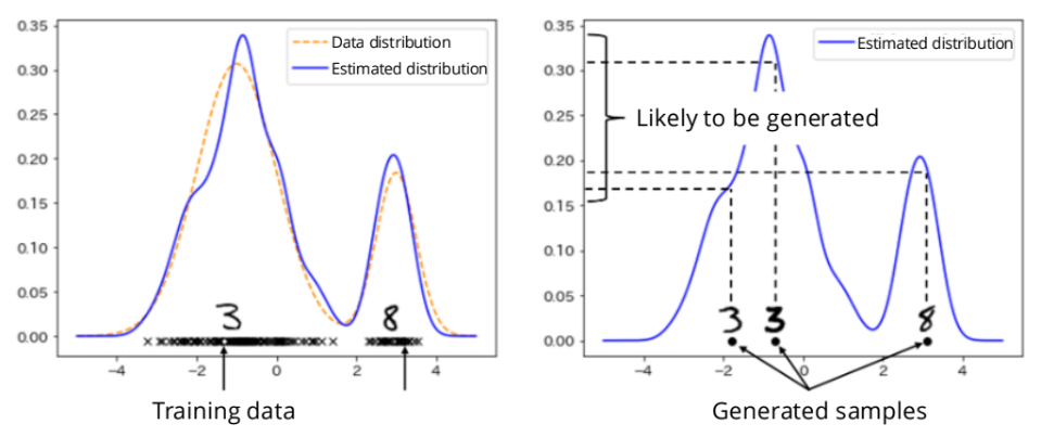
Another example, Generative AI. Training the model entails analyzing existing examples to find the underlying probability distribution that generated them. Then during generation phase, the model draws new data samples from those estimated distributions. This random sample becomes a brand-new, synthetic image or piece of text that looks authentic because it follows the probability rules of the original data.

7.4.1 Maximum Likelihood Estimation (MLE)

We want to find the parameter $\theta$ that makes the occurrence of $\{X_1, \dots, X_n\}$ as likely as possible, i.e. $$\max_{\theta} p_\theta(X_1, \dots, X_n)$$ Since we assume the observations are i.i.d., $$p_\theta(X_1, \dots, X_n) = \prod_{i=1}^{n} p_\theta(X_i)$$ If $n$ is huge, this number is very small and computers cannot handle it. Hence we take logarithm (recall the property $\log(A \times B) = \log A + \log B$).
Hence, MLE is solving for $$\max_{\theta\in\Theta}\sum_{i=1}^{n}\log p_{\theta}(X_{i})$$ For very complex distributions (like deep neural networks), solving this maximization problem directly is often impossible (intractable).
Hence, use approximation methods like EM algorithm, variational Bayes / variational autoencoders (VAEs), diffusion models.

7.4.2 Kullback–Leibler (KL) divergence

KL divergence is a statistical measure that quantifies how one probability distribution differs from a second, reference probability distribution.
In estimation context, KL divergence shows how closely our estimated model $q$ matches the true data distribution $p$.
For continuous probability densities $p$ and $q$, the KL divergence between them is $$D_{KL}(p||q) = \int p(x) \log \frac{p(x)}{q(x)} dx = \mathbb{E}_{X \sim p} \left[ \log \frac{p(X)}{q(X)} \right]$$ Two properties of KL divergence:

1. Non-negativity: $D_{KL}(p||q) \ge 0$.

2. Identity: $D_{KL}(p||q) = 0$ if and only if the two distributions are identical ($p = q$).

7.4.3 Connection between MLE & KL divergence

From the standard MLE sum, multiply by $\frac{1}{n}$ to get the empirical average: $$\max_{\theta} \frac{1}{n} \sum_{i=1}^{n} \log p_{\theta}(X_{i})$$ As $n \to \infty$, the empirical average converges to the theoretical expected value over the true data distribution $p$, by Law of Large Numbers, $$\max_{\theta} \mathbb{E}_{X \sim p}[\log p_{\theta}(X)]$$ To connect this to KL divergence, first subtract a constant. $$\begin{align*} \mathbb{E}_{X \sim p}[\log p_{\theta}(X)] &\sim \mathbb{E}_{X \sim p}[\log p_{\theta}(X)] - \mathbb{E}_{X \sim p}[\log p(X)] \\ &= \mathbb{E}_{X \sim p}\left[ \log \frac{p_{\theta}(X)}{p(X)} \right] \\ &= -D_{KL}(p || p_{\theta}) \end{align*}$$ Maximising the log-likehood minimises the KL divergence.

7.4.4 Example - Bernoulli Distribution

Given random variable $X \sim Ber(\theta)$, $P_\theta(X = 1) = \theta$, $P\theta(X = 0) = 1 - \theta$, $$P_\theta(X) = \theta^X \cdot (1 - \theta)^{1 - X}$$ Observations are $X_i \sim P$, ($i = 1, 2, \ldots, n$), which are i.i.d. The likelihood function is $$L(\theta) = \prod_{i=1}^{n} \theta^{X_i} (1-\theta)^{1-X_i}$$ Since the product is hard to calculate, the log likelihood function is $$\mathcal{L}(\theta) = \sum_{i=1}^{n} \left[ X_i \log(\theta) + (1-X_i) \log(1-\theta) \right]$$ To find $\theta$ that maximises the function, take the derivative wrt $\theta$ and set to 0: $$\frac{d\mathcal{L}}{d\theta} = \frac{1}{\theta} \sum_{i=1}^{n} X_i - \frac{1}{1-\theta} \sum_{i=1}^{n} (1-X_i) = 0$$ Solving, we get $$\hat{\theta} = \frac{1}{n} \sum_{i=1}^{n} X_i$$ The most optimal way to estimate the probability here is just the sample mean.
For example, given 10 coin flips, $D = \{1, 1, 0, 1, 1, 1, 0, 1, 1, 0\}$, $\hat{\theta} = 0.7$.
Interpretation: The parameter that makes this specific dataset the most mathematically likely to occur is $\theta = 0.7$.

Is this estimator efficient? (has the lowest possible variance)
For a Bernoulli distribution, the variance of a single trial $X_i$ is known to be $\mathbb{V}[X_i] = \theta_*(1-\theta_*)$. Then, $$\begin{align*} \mathbb{V}[\hat{\theta}] &= \mathbb{V}\left[\frac{1}{n}\sum_{i=1}^n X_i\right] \\ &= \frac{1}{n^2} \sum_{i=1}^n \mathbb{V}[X_i] \\ &= \frac{\theta_*(1-\theta_*)}{n} \end{align*}$$ We start with the log-likelihood of a single Bernoulli trial: $$\log P(X|\theta_*) = X\log(\theta_*) + (1-X)\log(1-\theta_*)$$ Using the definition of Fisher information: $$\begin{align*} \mathcal{I}(\theta_*) &= \mathbb{E}\left[\left(\frac{\partial}{\partial \theta_*} \log P(X|\theta_*)\right)^2\right] \\ &= \mathbb{E}\left[\left(\frac{X}{\theta_*} - \frac{1-X}{1-\theta_*}\right)^2\right] \\ &= \mathbb{E}\left[\frac{X^2}{\theta_*^2} - 2\frac{X(1-X)}{\theta_*(1-\theta_*)} + \frac{(1-X)^2}{(1-\theta_*)^2}\right] \\ &= \mathbb{E}\left[ \frac{X}{\theta_*^2} - 0 + \frac{1-X}{(1-\theta_*)^2} \right] \\ &= \frac{\mathbb{E}[X]}{\theta_*^2} + \frac{\mathbb{E}[1-X]}{(1-\theta_*)^2} \\ &= \frac{\theta_*}{\theta_*^2} + \frac{1-\theta_*}{(1-\theta_*)^2} \\ &= \frac{1}{\theta_*(1-\theta_*)} \end{align*}$$ Then the Cramér-Rao Lower Bound is: $$\begin{align*} \text{CRLB} &= \frac{1}{n \cdot \mathcal{I}(\theta_*)} \\ &= \frac{1}{n \cdot \left(\frac{1}{\theta_*(1-\theta_*)}\right)} \\ &= \frac{\theta_*(1-\theta_*)}{n} \\ &= \mathbb{V}[\hat{\theta}] \end{align*}$$ The implication: $\hat{\theta} = \frac{1}{n}\sum X_i$ is an efficient estimator.

7.4.5 Example - Multivariate Gaussian Distribution

Moving from just a single variable $x$, we now consider data points in $d$-dimensional space $\mathbb{R}^d$.
Define the mean vector $\mu$, which is a vector that contains the average value for every single dimension, and $\mu = \mathbb{E}_{X \sim p_\theta}[X]$.
Also, define the covariance matrix $\Sigma \in \mathbb{R}^{d \times d}$, which is a square matrix that captures the variance. Here, $\Sigma = \mathbb{E}_{X \sim p_\theta}[(X - \mu)(X - \mu)^\top]$. It tells us the variance of each individual dimension and how all the dimensions correlate with one another.
Recall the $d$-variate Gaussian PDF: $$p_\theta(x) = \frac{1}{(2\pi)^{d/2}\sqrt{\det \Sigma}} \exp\left(-\frac{1}{2}(x - \mu)^\top \Sigma^{-1} (x - \mu)\right)$$ with the normalisation constant in the front, and the term in the exponent calculating the "distance" of point $x$ from the mean $\mu$, scaled by the covariance.
The goal is to use MLE to calculate $\mu$ and $\Sigma$ that best fit the data.
$$\begin{align*} \mathcal{L}(\mu, \Sigma) &= \log \prod_{i=1}^{n} \frac{1}{(2\pi)^{d/2} |\Sigma|^{1/2}} \exp\left(-\frac{1}{2}(X_i - \mu)^\top \Sigma^{-1} (X_i - \mu)\right) && \text{(Log of the joint PDF)} \\ &= \sum_{i=1}^{n} \left[ -\frac{d}{2}\log(2\pi) - \frac{1}{2}\log|\Sigma| - \frac{1}{2}(X_i - \mu)^\top \Sigma^{-1} (X_i - \mu) \right] && \text{(Log rules: product to sum)} \\ &= -\frac{nd}{2}\log(2\pi) - \frac{n}{2}\log|\Sigma| - \frac{1}{2}\sum_{i=1}^{n} (X_i - \mu)^\top \Sigma^{-1} (X_i - \mu) && \text{(Factor constants out of sum)} \end{align*}$$ $$(\hat{\mu}, \hat{\Sigma}) = \arg\max_{\mu \in \mathbb{R}^d, \Sigma \in \mathbb{R}^{d \times d}} -\frac{n}{2}\log(\det\Sigma) - \frac{1}{2}\sum_{i=1}^{n}(X_i - \mu)^\top\Sigma^{-1}(X_i - \mu)$$ Taking derivative of this function w.r.t. to $\mu$ and $\Sigma$ and setting it to zero,

• $\hat{\mu} = \frac{1}{n}\sum_{i=1}^{n}X_i$

• $\hat{\Sigma} = \frac{1}{n}\sum_{i=1}^{n}(X_i - \hat{\mu})(X_i - \hat{\mu})^\top$

Conclusion: Applying MLE to a multivariate Gaussian distribution gives us the sample mean and the sample covariance matrix as our optimal estimators. As the number of samples increases, these calculated estimates will converge to the true, underlying parameters $\mu$ and $\Sigma$ of the distribution.

7.5 Bayesian Inference

Methods like MLE treated the parameter $\theta$ as a fixed, absolute, but unknown constant to solve for.
Bayesian Inference instead considers a probability distribution of $\theta$. $\theta$ is treated a random variable with its own probability distribution, and we can update our entire belief about the parameter as we gather more data.
The probabilistic structure is:

• Prior Distribution, $p(\theta)$: initial belief about the distribution of the parameter before you have observed any data.

• Likelihood, $p(x|\theta)$: how likely you are to observe the data $x$, assuming a specific parameter $\theta$ is true.

• Joint Distribution, $p(x, \theta) = p(x|\theta)p(\theta)$: combined probability of both the parameter and the data occurring.

The goal is to infer $\theta$ by calcuting the posterior distribution using Bayes’ Theorem: $$p(\theta|X_1, ..., X_n) = \frac{p(X_1, ..., X_n|\theta)p(\theta)}{p(X_1, ..., X_n)} = \frac{\prod_i p(X_i|\theta)p(\theta)}{\int \prod_i p(X_i|\theta')p(\theta')d\theta'}$$ The numerator can be written as the product of individual likelihoods since the observations are independent. The $\theta$ here represents the specific hypothesis we are currently testing.
The denominator calculates the total marginal probability of observing this specific set of data. We use the dummy variable $\theta'$ here to show that this integral sweeps across every possible value of the parameter to calculate a grand total. Because it integrates out the parameter, the denominator evaluates to a flat constant number.
With this updated belief, we want to make a prediction about new, unseen data. In other words, given all the past data observations $X_1, ..., X_n$ I have already seen, what is the probability of observing a completely new data point $x$?
We want to solve for $\hat{p}(x)$, the posterior predictive distribution. $$\hat{p}(x) = \mathbb{E}_{\theta\sim p(\theta|X_1, ..., X_n)}[p(x|\theta)]$$ The expected value is calculating the weighted average of the likelihood $p(x|\theta)$, where the "weights" are determined by how plausible each $\theta$ is according to your posterior distribution $p(\theta|X_1, ..., X_n)$.
Recall that if we used MLE, we would have calculated the single best parameter $\hat{\theta}_{MLE}$, and to predict a new data point, we just plug it into $p(x|\hat{\theta}_{MLE})$.

The expected value of a continuous function is found by integrating it over the probability distribution. Multiplying ($p(x|\theta)$) by the weights ($p(\theta|X_1, ..., X_n)$) and integrating over $\theta$, $$\begin{align*} \hat{p}(x) &= \int p(x|\theta) \cdot p(\theta|X_1, ..., X_n) d\theta \\ &= \int p(x|\theta) \left[ \frac{\prod_i p(X_i|\theta)p(\theta)}{\int \prod_i p(X_i|\theta')p(\theta')d\theta'} \right] d\theta \\ &= \frac{\int p(x|\theta) \prod_i p(X_i|\theta)p(\theta)d\theta}{\int \prod_i p(X_i|\theta')p(\theta')d\theta'} \end{align*}$$ Conclusion: Because Bayesian inference averages over all possible parameters rather than relying on a single estimate, its predictions are much safer, especially when you have very little data. If your dataset is small, your posterior distribution will be wide (highly uncertain). The integral naturally accounts for this uncertainty, preventing you from making overconfident predictions based on a small sample size. As you gather more data ($n \rightarrow \infty$), your posterior distribution becomes an incredibly narrow spike around the true parameter, and this massive integral mathematically simplifies down to become virtually identical to the MLE approach.

7.5.1 Bayesian Inference with Gaussian Distribution

Calculating that massive integral in the denominator to find the posterior is often computationally impossible for complex distributions.
Instead, we can the use a property of Gaussians: if your prior is a Gaussian, and your likelihood is a Gaussian, your resulting posterior is guaranteed to also be a Gaussian.
First, model the prior and likelihood by Gaussian distributions:

• The Prior, $\theta \sim \mathcal{N}(\mu_0, \sigma_0^2)$: Before seeing any data, you believe the true parameter $\theta$ is somewhere around $\mu_0$, but you have some uncertainty, represented by the variance $\sigma_0^2$.

• The Likelihood ($X_i \sim \mathcal{N}(\theta, \sigma^2)$): Observing data points $X_1, ..., X_n$, under the assumption that these data points are generated by a Gaussian distribution centered around the true parameter $\theta$, with a known variance of $\sigma^2$.

After observing $n$ data points, the belief updates. The posterior variance $\hat{\sigma}_n^2$ and posterior mean $\hat{\mu}_n$ are $$\hat{\sigma}_n^2 = \frac{\sigma^2 \sigma_0^2}{n\sigma_0^2 + \sigma^2} \quad \hat{\mu}_n = \frac{\sigma^2\sigma_0^2}{n\sigma_0^2 + \sigma^2} \left( \frac{\sum_{i=1}^{n}X_i}{\sigma^2} + \frac{\mu_0}{\sigma_0^2} \right)$$ As $n \to \infty$, $$\lim_{n \rightarrow \infty} \hat{\sigma}_n^2 = 0 \quad \lim_{n \rightarrow \infty} \hat{\mu}_n = \frac{\sum_{i=1}^{n}X_i}{n}$$ The uncertainty drops to 0, and the mean becomes exactly equal to the sample mean, ignoring the initial belief.

Conclusion: Recall that the sample mean $\frac{\sum X_i}{n}$ is the exact solution you get when you use MLE.
Bayesian Inference is asymptotically equivalent to MLE.
In small data regime (we have little data), MLE is vulnerable to extreme outliers and overfitting. Bayesian inference instead anchors the prediction to your prior belief.
In large data regime, the sheer volume of evidence overwhelms whatever initial bias or belief you had. The prior’s influence vanishes, and the Bayesian approach perfectly mathematically aligns with the Frequentist (MLE) approach.

7.5.2 Maximum a Posteriori Estimation

In Bayesian inference, the perfect way to make a prediction is to calculate $\hat{p}(x) = \mathbb{E}_{\theta \sim p(\theta|X_1, ..., X_n)}[p(x|\theta)]$.
However, this is intractable. This means that for complex, real-world models (like deep neural networks), the integrals required to calculate the full posterior and the expected value are too complicated and computationally heavy for a computer to actually solve.
Instead of averaging all possible parameters, MAP Estimation simply finds the single most likely parameter value at the very peak of the posterior distribution curve.
This value is denoted as $\hat{\theta}_{MAP}$, and it is found by taking the $\arg\max$ of the posterior: $$\hat{\theta}_{MAP} = \arg\max_\theta p(\theta|X_1, ..., X_n)$$ Specifically, the core MAP equation is $$\max_{\theta \in \Theta} \left\{ \sum_{i=1}^n \log p(X_i|\theta) + \log p(\theta) \right\}$$ There are two distinct parts in this equation:

1. The data likelihood $\sum_{i=1}^n \log p(X_i|\theta)$: This is the same log-likelihood term we maximized in standard Maximum Likelihood Estimation (MLE). It pushes the model to pick parameters that fit the observed data well.

2. The prior as a penalisation term $\log p(\theta)$: This is the log of your prior distribution acting as a penalisation term. If the MLE part tries to pick an extreme parameter that perfectly fits the data but goes against your initial beliefs, this prior term will mathematically penalize (reduce) the overall score.

Because of this added prior term, this problem is also called penalized maximum likelihood estimation.
Also, as $n \to \infty$, the data likelihood term (which is a sum) becomes massive, completely overwhelming the single, static $\log p(\theta)$ prior term. With enough data, MAP becomes identical to MLE.

After finding this single best parameter, we can use it to make predictions as $p(x|\hat{\theta}_{MAP})$.
MAP uses Bayesian logic (incorporating a prior belief) but outputs a single parameter like the Frequentist MLE approach.